
ENGINEERING MATHEMATICS III - PowerPoint PPT Presentation
1 / 189
Title:
ENGINEERING MATHEMATICS III
Description:
Obtain the iterative formula for finding the square root. of N and find. f(x) = x2 N f'(x) = 2x ... the given heights in feet above the. earths surface. ... – PowerPoint PPT presentation
Number of Views:599
Avg rating:3.0/5.0
Title: ENGINEERING MATHEMATICS III
1
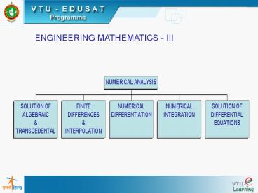
ENGINEERING MATHEMATICS - III
2
(No Transcript)
3
Numerical Analysis
Introduction
Limitations of analytical methods led to the
evolution of Numerical methods. Numerical Methods
often are repetitive in nature i.e., these
consist of the repeated execution of the same
procedure where at each step the result of the
proceeding step is used. This process known as
iterative process is continued until a desired
degree of accuracy of the result is obtained.
4
Solution of Algebraic and Transcendental
Equations The equation f(x) 0 said to be
purely algebraic if f(x) is purely a polynomial
in x. If f(x) contains some other functions like
Trigonometric, Logarithmic, exponential etc. then
f(x) 0 is called a Transcendental equation.
Ex (1) x4 - 7x3 3x 5 0 is algebraic
(2) ex - x tan x 0 is transcendental
5
Bisection Method This method is used in
locating a root of the equation f(x) 0 between
a and b. If f(x) is continuous
between a and b, f(a) and f(b) are opposite in
sign then exists a root between a and b. For
simplicity, let f(a) lt 0 and f(b) gt 0 The first
approximation to the root is If f(x1) 0 then
x1 is the root of f(x) 0 If f(x1) is ve then
root lies between a and x1 and the second
approximation to the root is
6
Now if f(x2) is - ve then the root lies between
x2 and x1 and the third approximation to the
root is This process is continued until the
root is found with desired accuracy
7
Problem 01
Solve x3 - 9x 1 0 for the root lying between
2 and 3 using bisection method in six
stages. f(x) x3 - 9x 1 0 f(2) -9
-ve f(3) 55 ve ? Root lies between
2.5 and 3
Solution
8
f(x2) f(2.75) -2.9 -ve ?
Root lies between 2.75 and 3
f(x3) 2.875 -1.111 -ve ? Root
lies between 2.875 and 3
f(x4) -0.09 -ve
? Root lies between 2.9375 and 3
f(x5) 0.451 ve ? Root lies
between 2.9375 and 2.969
9
f(x5) 0.17 ve ?
Root lies between 2.9375 and 2.953
10
Method of false position or Regula-Falsi
Method This is a method of finding a real root
of an equation f(x) 0 and is slightly an
improvisation of the bisection method. Let x0
and x1 be two points such that f(x0) and f(x1)
are opposite in sign.
11
Let f(x0) gt 0 and f(x1) lt 0 \ The graph of y
f(x) crosses the x-axis between x0 and x1 ?
Root of f(x) 0 lies between x0 and x1 Now
equation of the Chord AB is
When y 0 we get x x2
12
- Which is the first approximation
- If f(x0) and f(x2) are opposite in sign then
second approximation - This procedure is continued till the root is
found with desired accuracy.
13
Problem 02
Find a real root of x3 - 2x -5 0 by method of
false position correct to three decimal places
between 2 and 3.
Solution
- Let f(x) x3 - 2x - 5 0 f(2) -1
f(3) 16 - a root lies between 2 and 3
- Take x0 2, x1 3 ? x0 2, x1 3
14
2.0588 f(x2) f(2.0588)
-0.3908 ? Root lies between 2.0588 and 3
Taking x0 2.0588 and x1 3 f(x0) -0.3908,
f(x1) 16 Repeating the process the successive
approximations are x5 2.0915, x6 2.0934, x7
2.0941, x8 2.0943 Hence the root is 2.094
correct to 3 decimal places.
15
2.0813 f(x3) f(2.0813)
-0.14680 ? Root lies between 2.0813 and
3 Taking x0 2.0813 and x1 3 f(x0)
0.14680, f(x1) 16
16
Problem 03
Find the root of the equation xex cos x using
Regula falsi method correct to three decimal
places.
Solution
Let f(x) cosx - xex Observe f(0)
1 f(1) cos1 - e -2.17798 ? root lies
between 0 and 1 Taking x0 0, x1 1 f(x0)
1, f(x1) -2.17798
17
f(x2) f(0.31467) 0.51987 ve ? Root lies
between 0.31467 and 1 x0 0.31467, x1
1 f(x0) 0.51987, f(x1) -2.17798
18
f(x3) f(0.44673) 0.20356 ve ? Root lies
between 0.44673 and 1
Repeating this process x5 0.50995, x6
0.51520, x7 0.51692, x8 0.51748 x9
0.51767, etc Hence the root is 0.518 correct to
4 decimal places
19
Newton Raphson Method This method is used to
find the isolated roots of an equation f(x) 0,
when the derivative of f(x) is a simple
expression. Let m be a root of f(x) 0 near
a. ? f(m) 0 We have by Taylor's series
Ignoring higher order terms f(m) f(a)
(m - a) f' (a) 0
20
Let a x0, m x1
21
Problem 04
Using Newton's Raphson Method find the real root
of x log10 x 1.2 correct to four decimal
places.
Solution
Let f(x) x log10 x - 1.2 f(1) -1.2, f(2)
-0.59794, f(3) 0.23136
22
Let x0 2.5 (you may choose 2 or 3 also)
Repeating the procedure x3 2.7406
23
Problem 05
Using Newton's Method, find the real root of xex
2. Correct to 3 decimal places.
Solution
Let f(x) xex - 2 f(0) -2 f(1) e
- 2 0.7182 Let x0 1 f' (x)
(x 1) ex We have
24
Problem 06
Find by Newton's Method the real root of 3x
cosx 1 near 0.6, x is in radians. Correct for
four decimal places.
Solution
Let f(x) 3x - cosx - 1 f'(x) 3 sinx
Since x1 x2 . The desired root is 0.6071
25
Problem 07
Obtain the iterative formula for finding the
square root of N and find
Solution
? f(x) x2 N f'(x) 2x Now
26
Since x2 x3 6.4031
27
Problem 08
Obtain an iterative formula for finding the p-th
root of N and hence find (10)1/3 correct to 3
decimal places.
Solution
Let xp N or xp - N 0 Let f(x)
xp N f (x) pxp-1
? Use x0 2, p 3, N 10
28
(No Transcript)
29
Problem 09
Obtain an iterative formula for finding the
reciprocal of p-th root of N. Find (30)-1/5
correct to 3 decimal places.
Solution
Let x -p N or x -p - N 0 ?
f(x) x -p N f'(x) -px -p - 1 Now
We use x0 0.5, p 5, N 30
30
Finite Differences Forward difference operator
(D) ?f(x) f(x h) - f(x) ?yr y r 1 -
yr, r 0, 1, 2, , n -1
31
first forward differences
32
(No Transcript)
33
Difference Table
?y0, ?2y0, ?3y0,. are called the leading
differences
34
Ex The following table gives a set of values
of x and the corresponding values of y f(x)
Form the difference table and find ?f (10), ?2f
(10), ?3f (20) ?4f (15)
35
(No Transcript)
36
Note The nth differences of a polynomial of n
the degree are constant.
If f(x) a0 xn a1 xn-1 a2 xn-2 an, a0 ?
0 then
37
(No Transcript)
38
If y0 1, y1 11, y2 21, y3 28, y4 29.
Construct the difference table.
39
Backward difference operator (?)
Let y f(x) We define ?f(x) f(x) - f(x -
h) i.e. ?y1 y1 - y0 ?y0 ?y2 y2 - y1
? y1 ' ' ?yn yn - yn-1 ? yn - 1
40
Note ly ?n f(x nh) ??n f(x)
41
Backward difference table
42
Example 1. Form the difference table for
and find ?y (30), ?2y (70), ?5y (90)
43
2. Given
Construct the difference table and write the
values of ?f (4), ?2f (4), ?3f (3)
44
(No Transcript)
45
Central Difference Operator (?)
46
Note 1
Note 2
47
Central difference table
48
Problem
1. Show that
Solution
49
Problem
2. Show that
Solution
50
Problem
3. Given f(-2) 12, f(-1) 16, f(0) 15, f(1)
18, f(2) 20 form the central difference
table and write down the values of ?y-3/2,
?2y0, ?3y1/2 by taking x0 0
51
Solution
52
Shift operator (E)
E f(x) f(x h) E2 f(x) f(x 2h) En f(x)
f(x nh)
53
Note 1
Note 2
54
Interpolation
The word interpolation denotes the method of
computing the value of the function y f(x) for
any given value of x when a set (x0, y0), (x1,
y1),(xn-1, yn-1) are given.
Note Since in most of the cases the exact form
of the function is not known. In such cases the
function f(x) is replaced by a simpler function
?(x) which has the same values as f(x) for x0,
x1, x2.,xn-1.
55
is called the Newton Gregory forward difference
formula
- Note
- Newton forward interpolation is used to
interpolate the values of y near the beginning of
a set of tabular values. - y0 may be taken as any point of the table but
the formula contains those values of y which come
after the value chosen as y0.
56
Problem
The table gives the distances in nautical miles
of the visible horizon for the given heights in
feet above the earths surface.
Find the values of y when i) x 120, ii) y
218
57
Solution
Choose x0 100
58
i)
59
ii) Let x 218, x0 200,
15.7
60
2. Find the value of f(1.85)
61
(No Transcript)
62
Problem
Given sin 45o 0.7071, sin 50o 0.7660, sin
55o 0.8192, sin 60o 0.8660. Find sin 48o.
63
Solution
64
Problem
From the following data find the number of
students who have obtained ? 45 marks. Also
find the number of students who have scored
between 41 and 45 marks.
65
Solution
66
f(45) - f(40) 70 Number of students who have
scored between 41 and 45.
67
Problem
Find the interpolating polynomial for the
following data f(0) 1, f(1) 0, f(2) 1,
f(3) 10. Hence evaluate f(0.5)
68
Solution
f(0.5) 0.625
69
Problem
Find the interpolating polynomial for the
following data
70
(No Transcript)
71
Newton Gregory Backward Interpolation formula
72
Problem
The values of tan x are given for values of x in
the following table. Estimate tan (0.26)
73
Solution
74
(No Transcript)
75
Problem
The deflection d measured at various distances x
from one end of a cantilever is given by the
following table. Find d when x 0.95
76
Solution
77
Problem
The area y of circles for different diameters x
are given below
Calculate area when x 98
78
Solution
y 7542
79
Problem
Find the interpolating polynomial which
approximates the following data.
80
Solution
81
Central Difference Interpolation Formulae
Bessels and Stirlings are two of the central
difference interpolation formulae. These are used
to find y at a value of x that is in the
middle of x0 and xn
82
Central difference interpolation formula
83
a) Stirlings formula
84
b) Bessel's formula
85
Problem
Apply sterling's formula to find f(14.2) from
the following table
86
Solution
87
Problem
Apply stirling's formula to find a polynomial
f(x) of degree 4 that approximates the following
data and hence find f(2.5)
88
Solution
89
(No Transcript)
90
Problem
Using Bessels formula find f(12.5) for the data
91
Solution
92
Problem
Using Bessel's formula find 3rd degree
polynomial that approximates the following
data f(0) 2, f(1) 3, f(2) 8, f(3) 23
93
Solution
94
Interpolation with unequal intervals
Newton backward and forward interpolation is
applicable only when x0, x1,,xn-1 are equally
spaced.
Now we use two interpolation formulae for
unequally spaced values of x.
95
i. Lagranges formula for unequal intervals If
y f(x) takes the values y0, y1, y2,.,yn
corresponding to x x0, x1, x2,,xn then
96
is known as the lagrange's interpolation formula
97
ii) Divided differences (?)
98
second divided difference
99
Newton's divided difference interpolation formula
Newton backward and forward interpolation is
applicable only when x0, x1,,xn-1 are equally
spaced.
is called the Newton's divided difference formula.
100
Note Lagrange's formula has the drawback that
if another interpolation value were inserted,
then the interpolation coefficients need to be
recalculated. Inverse interpolation Finding
the value of y given the value of x is called
interpolation where as finding the value of x for
a given y is called inverse interpolation. Sinc
e Lagrange's formula is only a relation between x
and y we can obtain the inverse interpolation
formula just by interchanging x and y.
101
is the Lagranges formula for inverse
interpolation
102
Problem
The following table gives the values of x and y
Find x when y 12 using Lagranges inverse
interpolation formula.
103
Solution
Using Langrages formula
3.55
104
Problem
Given the values
Evaluate f(9) using (i) Lagrange's formula
(ii) Newton's divided difference formula
105
Solution
i) Lagranges formula
106
(No Transcript)
107
(ii) Newton's divided difference formula
f(9) 150 121 (9 - 5) 24 (9 - 5) (9 - 7)
1(9 - 5) (9 - 7) (9 - 11) 810
108
Problem
Using i) Langranges interpolation and ii)
divided difference formula. Find the value of y
when x 10.
109
Solution
Lagranges formula
110
Divided difference
111
(No Transcript)
112
Problem
If y(1) -3, y(3) 9, y(4) 30, y(6) 132 find
the lagranges interpolating polynomial that
takes the same values as y at the given
points. Given
113
Solution
114
Problem
Find the interpolating polynomial using Newton
divided difference formula for the following
data
115
Solution
F(x) 2 (x - 0)(1) (x - 0) (x - 1) (4) (x
- 0) (x - 1) (x - 2) 1 x3 x2 - x 2
116
Central Difference Interpolation Formulae
1.Find y(35) given y(20) 5/2, y(30) 439,
y(40) 346 and y(50) 243 We get the
following difference table
xp x0 ph ? 35 3010p ? p 0.5
?y(35) 439
394.375.
117
Examples
2. Find the third degree polynomial that
approximates the function f(x) given by f(0)
2, f(1) 3, f(2)8 f(3) 23. Hence find
f(1.5) f(2.3). The difference table is given
by
118
xp x0 ph ? x 1p ? p x - 1
f(x) x3 x2 x 2 is the polynomial.
? f(1.5) 4.625 and f(2.3) 11.177
Note Bessels formula gives better results when
there are an even number of
observations
119
Example
.
Find the population of a town (in appropriate
units) for the year 1974 given that
120
- The difference table for the data is given below
121
- xp x0 ph ? 1974 1969 10p ? p 0.5
?
y (1974) 32.461
Note Stirlings formula is used when an odd
number of observations is given.
122
1. Find f(4) given f(0) -4, f(2) 2, f(3)
14 and f(6) 158 The divided difference
table is
? f(4) -4 (4 ) (3) (4) (2) (3) (4) (2)
(1) (1) 40
123
2. Fit an interpolating polynomial for u4
48, u5 100, u6 180 , u8 448, u10 900 and
u11 1210
The table of divided differences is
? y 48 (x -4) 52 (x-4) (x-5) 14 (x-4)
(x-5) (x -6) x3- x2
124
Examples
1. Find u5 if u0 1, u319, u449, u6 181
At x 5, u is given by
125
Examples
2. Fit a polynomial x f(y) for the data
The polynomial, using Lagranges inverse
interpolation formula, is given by
? x y2 1 is the required polynomial
126
Examples
3. Apply Lagranges formula and obtain the root
of f (x) 0 if f(30) -30,
f(34) -13, f(38) 3 and f(42) 18 The
data can be arranged in the form
127
Numerical Differentiation
128
NUMERICAL DIFFERENTIATION
Numerical differentiation is the determination of
approximate values of the derivatives of a
function f(x) that is given by a table of
values. When the values of y (a function of x)
at some equally spaced values of x are known,
approximate values of f (x), f(x) and so on
can be calculated by numerical methods using
interpolation formulas.
129
If y0, y1, yn are the values of y
corresponding to x0, x1....xn (equally
spaced) then
at x x
0,
130
Note 1. The above formulae are got by
differentiating Newtons forward
and backward difference interpolation formulae
w.r.t. p and using
2. If f (x) and f (x) are
to be found at a tabulated value
of x, the value of p is chosen to be 0 in the
formulae.
otherwise p is given by
or
according as x lies close to x0 or xn
respectively.
131
Examples
1. Find y (0) and y (0) from the given
table
132
Forming the difference table, we get
We have h 1 ? f (0) - 27.9
and f (0) 117.67
133
Examples
2. The population of a certain town is shown
below . Estimate the rate of growth of
population in the year 1951
134
- The above data, after rearranging, we get
Here h 10 . We get the rate of growth of
population as
135
NUMERICAL INTEGRATION
136
Numerical Integration
The process of evaluating a definite integral of
the form
where a b are given and f(x) is a function
given analytically by a formula or
empirically by a table of values.
137
Geometrically, I is the area under the curve
f(x ) between x a and x b.
The method here is to approximate the integrand
f(x) by polynomials. The given interval (a ,
b) is divided into a number of subintervals of
equal width (say h). Replacing f(x) by
polynomials of different degrees lead to
different rules of integration.
138
Numerical Integration
139
Rules of integration
Trapezoidal rule
Approximating f(x) by a piecewise linear
function, we obtain the Trapezoidal rule given
by
y
where b a nh and n
is an integer
140
y
a x0 x1 x2
xn-1
xn b Trapezoidal Rule
x
0
x
141
Examples
1. Evaluate
, choosing 7 ordinates.
Hence find an approximation for ln 2.
7 ordinates implies 6 subintervals.
? h , width of a subinterval 1/6
we have the following table of values
142
Examples
Trapezoidal rule gives
ln 2
But
?
ln 2 ? 0.2316 or ln 2 ? 0.6948
143
Examples
choosing subintervals of equal width
2. Evaluate
Compare with the theoretical value.
Here y f(x) cosx, h
The table of values is
144
Examples
By Trapezoidal rule,
But
? The error is ? 0.002
145
Simpsons One Third Rule
Approximating f(x) by a piecewise quadratic
function gives Simpsons one third rule
Here the number of subintervals is a multiple of
2.
146
Simpsons One Third Rule
y
0
x
a x0 x1 x2 x3 x4 - - - - -
- - - - x2n-2
x2n-1 x2nb Simpsons rule
147
Examples
1. Evaluate
by dividing the interval (0,1) into 4
equal subintervals
and hence find the value of ?
correct to four decimal places.
. The table of values is
f(x)
h
148
By Simpsons rule
But
? ? ? 4 (0.7854) 3.1416, correct to four
decimal places.
149
Simpsons Three Eighth Rule
The integrand f(x), when approximated by a
piecewise cubic function, the required integral
reduces to
This is Simpsons three eighth rule. Here the
number of subintervals is a multiple of 3.
150
Examples
Evaluate
taking 6 equal strips and hence
find an approximation for ? .
Here h 1/6, with this the following table
is formed
151
Examples
By Simpsons 3/8th rule, the given integral is
equal to
But
?/6
- Using Simpsons 3/8th rule, an approximate value
of - ? is 3.1416.
152
Weddles Rule
Weddles rule of integration is obtained when
f(x) is approximated by a piecewise sixth degree
function and is given by
Here the number of subintervals is a multiple
of 6.
Note Among all the four rules, Simpsons one
third rule is sufficiently accurate
for most of the problems.
153
Examples
1. Evaluate
choosing 7 ordinates.
Compare with the theoretical value.
h 1/6 gives the following table of values
154
Examples
By Weddles rule, the integral is
But
- The value of the integral is correct to 4
decimal places - by Weddles rule.
Note 1. Simpsons one third rule gives 0.5009
2. Simpsons three eighth rule
gives 0.50018
155
Examples
2. Evaluate
using all the four rules and
compare with the exact value 4.05095.
Let the number of subintervals be 6. Then h
0.2
Letting y sin x ln x ex, the values
of xi and the corresponding yi are
tabulated as below
156
Examples
we get the value of the given integral as
4.07146 by Trapezoidal,
4.05208 by Simpsons 1/3rd ,
4.05293 by Simpsons 3/8th
and 4.05139 by Weddles rule.
We observe that Weddles rule gives the best
approximation compared to the other three rules.
157
Numerical Solution of first
Order ODE
158
Numerical Solution of first Order ODE
- There are various numerical methods to solve the
initial value - problem
The methods yield solutions either as power
series in x or directly as a numeric at a given
x. Here we study four numerical methods.
159
Methods of solution
Runge-Kutta Fourth order
Milnes predictor-corrector
Eulers Modified method
Taylors series
160
Taylors Series Method
Given the problem
y(x) is expanded in the form of a Taylors series
about the point x x0 as
The value of y at any given x can be found by
substituting for y, y etc. using the given
equation. The above power series gives the
values of y for every x for which the
series converges.
161
Examples
1. Evaluate y(0.1) correct to six places of
decimals if y(x) satisfies y xy 1
y(0) 1. y xy 1 ? (y)(0) 1.
Differentiating y with reapect to x we get
y xy y ? y(0) 1 y
xy 2y ? y(0) 2 y(IV)
xy 3y ? y(IV) (0) 3 y(V)
xyIV 4y ? yv(0) 8 yVI xyv
5yIV ? yvI(0) 15
162
Examples
The Taylors series expansion for f(x) about
the point x x0 0 is
when x 0.1, y(0.1) 1.105347 correct to
6 decimal places.
163
Example
2. Solve y y2 x , y(0) 1 using
Taylors series method and compute y(0.1)
and y(0.2) Given y y2 x, y(0) 1
y 2yy 1 ? y(0)
3 y 2y2 2yy ? y(0)
8 yIV 6yy 2yy ? yIV (0) 34
Taylors series expansion for y(x) about the
point x 0, upto fourth degree terms is
? y (0.1) 1.116475 and y (0.2) 1.272933
164
Modified Eulers Method
This is a predictor - corrector method which
consists of two formulae predictor formula and
corrector formula. Given the problem
To find y at x x0 h, where h is a small
increment in x, follow the steps given below
165
Step 1 Estimate y, using the formula y1 y0
h f (x0, y0), called the predictor
formula
Step 2 Find
, first refined value of the estimate y1 using
the corrector formula given by
y0
166
Continue this refinement until we get
with y1(i) and y1(i-1) as equal (to the
desired accuracy) (the ith and the i-1th
corrections of y are equal).
167
Numerical Solution of first order ODE
Modified Eulers Method
Note 1. Predictor corrector method is the
technique of refining an initially
crude estimate of yi by means of
a more accurate formula. 2..This
method is a modification of Eulers method.
Here the predictor formula or Eulers
formula yi yi-1 h
f(xi-1, yi-1) is used to find successive
values of y. 3. Geometrically,
the curve in this method is
approximated by a line through the point (x0,
y0) having the slope as the
average of the slopes at (x0, y0)
and (x0h, y1) which is manifested in the
corrector formula.
168
Examples
- Apply 5 corrections of Eulers modified method to
- find an approximate value of y (0.1) for the
problem
Let h 0.1. Using the predictor formula, we get
y1 1.1 By corrector formula we get the
corrections y1(1) 1.09167 y1(2)
1.09161 The 3rd, 4th and 5th corrections give
1.09161
169
Examples
2. Given
y(1) 1, find an approximate value of
y at x 2 in steps of 0.2
First Step
y1 1 0.221 1.6
y1(1) 1 0.1 3 2
1.639
y1(2) 1 0.1 3 2
1.640
1.640
y1(3) 1 0.1 3 2
170
Second Step
x0 1.2, y0 1.640 ? f(x0, y0)
3.403 y1 1.64 0.2 (3.403) 2.3206
y1(1) 1.64 0.1 3.403 2
2.361
y1(2) 1.64 0.1 3.403 2
2.362
y1(3) 2.362
171
Third Step
- x0 1.4, y0 2.362 ? f(x0, y0)
3.818 - y1 2.362 0.2 (3.818) 3.126
3.167
y1(1) 2.362 0.1 3.818 2
y1(2) 3.169 y1(3)
172
Fourth Step
- x0 1.6, y0 3.169 ? f(x0, y0)
4.252 - y1 3.169 0.2 (4.252) 4.02
y1(1) 3.169 0.1 4.252 2
4.063
y1(2) 4.065 y1(3)
173
Modified Eulers Method
Examples
Fifth Step
- x0 1.8, y0 4.065 ? f(x0, y0)
4.705 - y1 4.065 0.2 (4.705) 5.006
y1 (1) 4.065 0.1 4.705 2
5.052
y1(2) 5.053 y1(3) ?y(2)
5.053
174
Runge Kutta Fourth Order Method
This numerical method, also referred to as
Runge-Kutta method, is a most commonly used
method to solve a linear as well as a non-linear
differential equation. This method does not
require higher order derivatives of the function.
To solve an initial value problem
in finding y at a given x.
Let x x0 h and the corresponding y
y0 k.
175
For a known h, k is found as the weighted
mean of the quantities k1, k2, k3 and k4
which are given by the formulae
k1 h f(x0, y0),
k2 h f(x0 h/2, y0 k1/2),
k3 h f(x0 h/2, y0 k2/2)
and k4 h f(x0 h, y0 k3)
k is computed using k (k1 2 k2 2
k3 k4 )/6.
176
Examples
1. Find y(0.2) given
choosing h 0.1.
Step1
x0 0, y0 1, h 0.1, f(x0, y0) 0.5 k1
(0.1)(0.5) 0.05
k2
k3
k4
? k 0.06653 ? y(0.1) 1 0.06653
1.06653
177
Step2
x0 0.1, y0 1.06653, h 0.1, f(x0, y0)
0.83327. k1 (0.1)(0.83327) 0.083327
k2
k3
k4
? k 0.10069 ? y (0.2) 1.1672.
178
Examples
2. Evaluate y(1.1) given
Let h 0.1, f(x,y)
x0 1, y0 1, f(x0, y0) 0
179
- k1 0.1 (0) 0
- 0.004535
k2
k3
- 0.004319
k4
- 0.007871
- k - 0.004263
- ? y(1.1) 0.9957
180
Milnes Method
This is a predictor- corrector method of solving
a differential equation that can be used to find
y at a given x, provided the previous four
consecutive values of y are known. The method is
explained below
Given
To find an approximate value of y at x xn
x0 nh.
181
Using y(x0) , compute y1 y(x0 h), y2
y(x02 h) and y3 y(x03 h), by any method (
Taylors series method can be used). Then
calculate f0 f (x0, y0), f1 f(x1,y1),
f2 f (x2, y2) and f3 f (x3, y3)
182
To find y4 y (x0 4h), use the predictor
formula
Now, let f4 f(x0 4h, y4)
The value of y4 is corrected using the
corrector formula y4 (c) y2 h/3
(f2 4 f3 f4)
183
Then an improved value of f4 is computed and
again the corrector is applied to improve y4.
This process is repeated until two consecutive
corrected values of y4 remain unchanged (to the
desired accuracy). The above procedure can be
continued to find further values of y.
184
Examples
1. Given
Find y(0.4) correct to 3 decimal places given
x 0.1 0.2 0.3 y
1.105 1.223 1.355
Form the table of values
185
Examples
Predict y4 by y0 4h/3 (2f1- f2 2f3)
1.579 ? f4 1.998
Correct y4 by y2 h/3 (f2 4 f3 f4)
First correction
Second correction
Third correction
? y(0.4) 1.538 correct to 3 decimal places
186
Examples
2. Use Milnes method to find y(0.3) from
y x2 y2 y(0)1
Find the initial values y(-0.1), y(0.1) and
y(0.2) using Taylors series method.
Here h0.1, x0, y1, f(x,y)x2 y2
y x2 y2 ? y(0)
1 y2x2yy ?
y(0) 2 y22y22yy ?
y(0) 8 y6yy 2yy ?
y(0) 28
187
Examples
Using Taylors series expansion,
y(0) . . . .
y(x) y(0) x.y(0)
y(0)
y(0)
x4 upto 4th degree terms.
x3
1 x x 2
?y(-0.1) 0.9088, y(0.1) 1.1114, y(0.2)
1.2525
188
Examples
Form the table of values
y4(p) y0 4h/3(2f1- f2 2f3)
1.4384 ? f4 2.1591, using x4 0.3
? first correction
1.43937 ? f4 2.1618
189
Examples
second correction
third correction
? y(0.3) 1.4395 correct to 4 decimal places.
Recommended
CrystalGraphics Presentations


