
Why an Antiproton source? - PowerPoint PPT Presentation
1 / 33
Title:
Why an Antiproton source?
Description:
p pbar physics with one ring Dense, intense beams for high luminosity Run II Goals 36 bunches of 3 x 10¹⁰ pbars Small energy spread Small transverse dimensions – PowerPoint PPT presentation
Number of Views:69
Avg rating:3.0/5.0
Title: Why an Antiproton source?
1
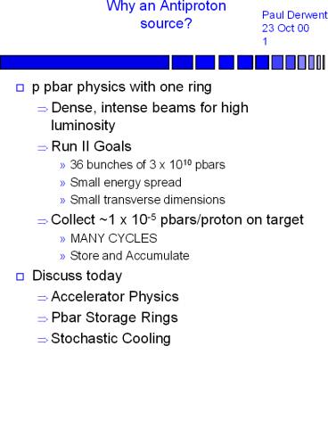
Why an Antiproton source?
- p pbar physics with one ring
- Dense, intense beams for high luminosity
- Run II Goals
- 36 bunches of 3 x 10¹⁰ pbars
- Small energy spread
- Small transverse dimensions
- Collect 1 x 10⁻⁵ pbars/proton on target
- MANY CYCLES
- Store and Accumulate
- Discuss today
- Accelerator Physics
- Pbar Storage Rings
- Stochastic Cooling
2
Some Necessary Accelerator Physics
- All Classical (Relativistic) EM
- Hamiltonian of a charged particle in EM field
- Small angle approximation around CENTRAL ORBIT
- Set of Conjugate variables
- x, x horizontal displacement and angle
- y, y vertical displacement and angle
- E, s energy and longitudinal position
- s bct sometimes use t instead
- Equation of Motion
- C is circumference of accelerator -- Periodicity!
3
Solutions to Equations of Motion
- Restoring force k(s) is dependent on location
- Dipoles
- Quadrupoles
- Drifts
- General Solution
- b(s) is solution to a messy 2nd order Diff Eqn
- Beam size depends on Amplitude of oscillation and
value of b(s) - Can change Position by changing angle 90?
upstreamused for extraction/injection/cooling/IP
position
4
Beam Size
- Relate the INVARIANT EMITTANCE (phase space area)
to physical size - Gaussian Beams
- 95 (Fermi Standard)
- s2 eb / 6p
- Include relativistic contraction (beams gets
smaller as they are accelerated!) - At B0 b(s) b(1s2/b2)
- For 20p mm mr beams at IP
- s (20p x10-6 m r 0.35 m / 6pg)1/2 3.5 x
10-5 m 35 mm
5
Longitudinal Effects
- Longitudinal Acceleration
- Time Varying Fields to get net acceleration
- Synchronous PHASE and Particle
- Path Length can depend on ENERGY
- Revolution Frequency can depend on ENERGY
- Expressed via Phase Slip Factor h
- gt transition energy
- Accelerating phase needs to change by 180 as
cross transition
6
Final Points
- Frequency Spectrum
- Time Domain ???(tnT0) at pickup
- Frequency Domainharmonics of revolution
frequency f0 1/T0 - AccumulatorT01.6 ?sec (1e10 pbar 1 mA)f0
(core) 628955 Hz - 127th Harmonic 79 MHz
7
Pbar Storage Rings
- Two Storage Rings in Same Tunnel
- Debuncher
- Larger Radius
- few x 107 stored for cycle length
- 2.4 sec for MR, 1.5 sec for MI
- few x 10-7 torr
- RF Debunch beam
- Cool in H, V, p
- Accumulator
- 1012 stored for hours to days
- few x 10-10 torr
- Stochastic stacking
- Cool in H, V, p
- Both Rings are triangular with six fold symmetry
8
Debuncher Ring
- Main Purpose
- Debunch RF Time Structure (84 buckets)RF
locked to Main Injector - Rotation in Phase Space
- DE, Dt conjugate variables
- Initial large DE (off target), small Dt (RF)
- 5 MV RF in 1/4 turn down to 100 kV
- Small DE, large Dt
- Adiabatically turn off RF (10 msec)
- Lots of time left (1.5 sec cycle)
- Cool in H, V, p
9
Accumulator Ring
- Not possible to continually inject beam
- Violates Phase Space Conservation
- Need another method to accumulate beam
- Inject beam, move to different orbit (different
place in phase space), stochastically stack - RF Stack Injected beam
- Bunch with RF (2 buckets)
- Change RF frequency (but not B field)
- ENERGY CHANGE
- Decelerates 30 MeV
- Stochastically cool beam to core
- Decelerates 60 MeV
10
Idea Behind Stochastic Cooling
- Phase Space compression Dynamic Aperture
Area where particles can orbit Liouvilles
Theorem Local Phase Space Density for
conservative system is conserved Continuous
Media Discrete Particles Swap Particles
and Empty Area -- lessen physical area
occupied by beam
11
Idea Behind Stochastic Cooling
- Principle of Stochastic cooling
- Applied to horizontal btron oscillation
- A little more difficult in practice.
- Used in Debuncher and Accumulator to cool
horizontal, vertical, and momentum distributions - COOLING? Temperature ltKinetic Energygtminimize
transverse KE minimize DE longitudinally
12
Stochastic Coolingin the Pbar Source
- Standard Debuncher operation
- 108 pbars, uniformly distributed
- 600 kHz revolution frequency
- To individually sample particles
- Resolve 10-14 seconds100 THz bandwidth
- Dont have good pickups, kickers, amplifiers in
the 100 THz range - Sample Ns particles -gt Stochastic process
- Ns N/2TW where T is revolution time and W
bandwidth - Measure ltxgt deviations for Ns particles
- Higher bandwidth the better the cooling
13
Betatron Cooling
- With correction gltxgt, where g is gain of system
- New position x - gltxgt
- Emittance Reduction RMS of kth particle
- Add noise (characterized by U Noise/Signal)
- Add MIXING
- Randomization effects M number of turns to
completely randomize sample
14
Momentum Cooling
- Momentum Cooling explained in context of Fokker
Planck Equation - Case 1 Flux 0 Restoring Force
a(E-E0) Diffusion D0 - Cooling of momentum distribution (as in
debuncher) - Small group with Ei-E0 gtgt D0
- Forced into main distribution
- MOMENTUM STACKING
15
Stochastic Stacking
- Gaussian Distribution
- CORE
- Injected Beam (tail)
- Stacked
16
Upgrades for Run II
- Debuncher
- All stochastic cooling systems
- Larger bandwidth (4-8 GHz vs. 2-4 GHz)
- All new electronics and signal transmission
- Lower Noise (Liquid Helium vs. Liquid Nitrogen)
- Different Technology
- Slot coupled waveguides vs. Octave bandwidth
pickups - Remove H V trim magnets to make room for
cooling tanks - Move quadrupoles for use in steering
- Adjust quad positions in D-to-A line to make room
for cooling tanks
17
Slot Coupled Waveguides
Output Port
Output Termination
Output Port
Output Termination
- Slot Coupled Waveguide an electromagnetic
whistle - Narrow Band (0.5 GHz), High Sensitivity
- Cover 4 bands (2 GHz bandwidth)
18
Debuncher Upgrade
- Slot Coupled Waveguide
- Narrow Band (0.5 GHz), High Sensitivity
- Cover 4 bands (2 GHz bandwidth)
19
Debuncher Upgrade
- Slow Wave Structure size, spacing, and number
of slots determines sensitivity and bandwidth
20
Debuncher Upgrades
- 4 Kicker bands
- 8 Pickup bands
21
Debuncher Momentum Cooling
- Beam on Accumulator Injection Orbit
- Blue Trace
- Debuncher Momentum
- Cooling Off
- Orange Trace
- Debuncher Momentum
- Cooling On
22
Debuncher Signal to Noise
- For Horizontal Band 1
- Signal to Noise for 1e7 particles (expect 8e7
during Run II) - Room Temperature (red), He Temperature
(blue/purple)
23
Stochastic Stacking
- Simon van Der Meer solution
- Constant Flux
- Solution
- Exponential Density Distribution generated by
Exponential Gain Distribution
Using log scales on vertical axis
24
Implementation in Accumulator
- Stacktail and Core systems
- How do we build an exponential gain distribution?
- Beam Pickups
- Charged Particles E B fields generate image
currents in beam pipe - Pickup disrupts image currents, inducing a
voltage signal - Octave Bandwidth (1-2, 2-4,4-8 GHz)
- Output is combined using binary combiner boards
to make a phased antenna array
25
Beam Pickups
- Pickup disrupts image currents, inducing a
voltage signal
26
Beam Pickups
- At ACurrent induced by voltage across
junction splits in two, 1/2 goes out, 1/2 travels
with image current
27
Beam Pickups
- At BCurrent splits in two paths, now
with OPPOSITE sign - Into load resistor 0 current
- Two current pulses out signal line
I
B
DT L/bc
28
Beam Pickups
- Current intercepted by pickup
- Use method of images
- Placement of pickups to give proper gain
distribution
w/2
-w/2
y
d
x
Dx
Current Distribution
29
Accumulator Pickups
- Placement, number of pickups, amplification are
used to build gain shape
Core A - B
Stacktail
Energy
Gain
Core
Stacktail
Energy
30
Accumulator Upgrades for Run II
- Accumulator
- Stacktail Stochastic Cooling Systems
- Larger Bandwidth (2-4 GHz vs. 1-2 GHz)
- New technologies for signal combination
- Recycled (from Debuncher) and new Electronics to
cover larger bandwidth - Lattice changes
- Halve phase slip factor (h)
- Driven by Stacktail upgrade
- Keep dispersion, phase advance (pickup to kicker)
injection and extraction regions, tunes,
aperture, chromaticity the same - Requires construction 4 new quadrupoles (strength
vs. current characteristics) - Reworking of power supplies
31
Why change h?
- ?f/f ???p/p h/DDx/x
- Momentum Spread100 MeV
- Frequency Spread 160 Hz
- fcentral 628900 Hz
- ?f /f 2.5e-4
- Stacktail assumes position(energy) frequency
relation in design - 1 GHz 1590 Harmonic
- ?f 254000 Hz
- 2 GHz 3180 Harmonic
- ?f 508000 Hz
- 3 GHz 4770 Harmonic
- ?f 763000 Hz
- Frequency Spread gt harmonic frequency!
- Frequency ? Energy Map no longer 1 ? 1
32
Accumulator Stacktail Performance with Protons
- Inject 8 GeV protons
- Stacking rate 13 mA/hour!
33
AntiProton Source
- Shorter Cycle Time in Main Injector
- Target Station Upgrades
- Debuncher Cooling Upgrades
- Accumulator Cooling Upgrades
- GOAL gt20 mA/hour