
Direct Migration of Passive Seismic Data - PowerPoint PPT Presentation
1 / 2
Title:
Direct Migration of Passive Seismic Data
Description:
Direct Migration of Passive Seismic Data Brad Artman1, Deyan Draganov2, Kees Wapenaar2, Biondo Biondi1 1Stanford Exploration Project, Geophysics, Stanford University ... – PowerPoint PPT presentation
Number of Views:46
Avg rating:3.0/5.0
Title: Direct Migration of Passive Seismic Data
1
Direct Migration of Passive Seismic Data
Brad Artman1, Deyan Draganov2, Kees Wapenaar2,
Biondo Biondi1 1Stanford Exploration Project,
Geophysics, Stanford University, 94305,
USA 2Department of Applied Earth Sciences, Delft
University of Technology, Mijnbouwstraat 120,
2628 RX, Delft, The Netherlands
Introduction
Intuition via incident plane-wave
If the integral over the boundary ?Dm, on which
the subsurface sources are situated, is
discretised and the subsurface sources are
assumed white and completely uncorrelated in
time, equation (1) can be rewritten as
General relations between the reflection and the
transmission responses of a 3-D inhomogeneous
medium 4 have been developed to forward model
the transmission coda, suppress multiples,
provide the basis of seismic interferometry, and
forward model the reflection response from the
transmission response. The final relation,
exploited for acoustic daylight imaging, shows
that by cross-correlating traces of the
transmission response of a medium one can
synthesize the reflection response collected in a
conventional active source experiment. Having
generated shot-gathers in this manner, they can
be processed with conventional techniques to
enhance signal, remove artifacts, or create a
migrated image. Here, we present the theory of
direct migration of the measured transmission
response wavefields without the need to first
generate the reflection response wavefields by
cross-correlation. Removing this step allows for
significant time savings when dealing with these
inherently large data sets and produces an
equivalent image. Apart from computational
advantages, moving the modeling of the reflection
response from the transmission response down to
the image point during migration opens the
possibility of more advanced imaging conditions
in the future.
Reflector
Free-surface reflection
Downward reflection
Incident plane wave
where Tobs is the collection of observed traces
that include all subsurface sources Ni
Free-surface reflection
Equations (3) and (4) are traces from the passive
recording of the ambient seismic energy within
the subsurface domain D observed at the surface
points A and B repsectively. In equation (2) the
noise sources are distributed along the surface
?Dm. However, the correlation process eliminates
the extra travel times related to different
source depths. This allows the sources to be
randomly distributed at or below the surface ?Dm
(see Figure 2).
Passive seismic imaging formulae
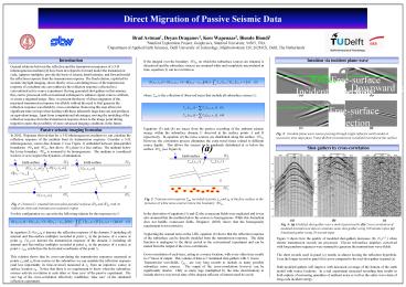
Fig. 3 Incident plane wave source passing
through single reflector earth model at
successive time steps (a-c). Panel d shows
transmission wavefield recorded at the surface.
In 2002, Wapenaar showed that for a 3-D
inhomogeneous medium we can calculate the
reflection response of the medium from its
transmission response. Consider a 3-D,
inhomogeneous, source-free domain D (see Figure
1) embedded between plan-parallel boundaries ?D0
and ?Dm. Just above ?D0 there is a free surface.
The medium below the lower boundary ?Dm is
assumed to be homogeneous. The medium is
considered lossless so as to neglect the dynamics
of attenuation.
(a)
Fig. 2 Transmission response Tobs recorded at
points xA and xB at the free surface in the
presence of white noise sources below the
boundary ?Dm.
Fig. 1 Domain D, situated between plan-parallel
surfaces ?D0 and ?Dm with its reflection (left)
and transmission response (right).
In the derivation of equations (1) and (2) the
evanescent fields were neglected and it was also
assumed that the medium below the sources is
homogeneous. While this formalism does not handle
evanescent fields, Draganov (2003) shows that the
homogenaity requirement is not restrictive. Negle
cting the acausal term on the LHS, equation (2)
shows that the reflection response of the
subsurface can be directly modeled from the
transmission response. The delta function is
analagous to the direct arrival in the
conventional experiment and can be muted from the
output of the cross-correlations. Cross-correlati
on of each trace, acting as a source location,
with every other trace results in N2 traces of
output. This volume of data is N simulated
shot-gathers with N traces. Transmission
wavefields, Tobs , are very long records to
include as many possible subsurface noise
sources. The ouput of the cross-correlations
however can be significantly shorter. Only as
many lags (multiplied by the time discritization)
to include the two-way-travel time of the deepest
reflector of interest need be saved.
For this configuration we can write the following
relation for the responses in D
In equation (1) R(xA,xB,t) denotes the reflection
response of the domain D including all internal
and free-surface multiples recorded at point xA
in the presence of a source at point xB.
T(xA,x,t) denotes the transmission response of
the domain D including all internal and
free-surface multiples recorded at point xA in
the presence of a source at point x. xH,A
symbolizes the horizontal coordinates of the
point A. This relation shows that by
cross-correlating the transmission responses
measured at points xA and xB from sources in the
subsurface we can simulate the reflection
response (and less importantly its time-reversal)
measured at xA from an impulsive source at
surface location xB. Notice that there is no
requirement to know when the subsurface sources
activate in relation to each other or time zero
of the passive experiment. The zero lag of the
cross-correlation effectively establishes time
zero of the simulated reflection experiment.
2
Using equation (2), we can calculate the
reflection response by cross-correlating one of
the transmission traces (in this case the trace
at horizontal position 0 m. see right picture
on Figure 4) with all the transmission traces
from the transmission panel. After muting the
non-causal part from the correlation result, we
receive the simulated reflection response as
shown on Figure 5 (left). The right picture on
the same figure shows for comparison the directly
modelled reflection response.
Fig. 6 (left) Simulated reflection response from
the right model on Figure 3 (right) directly
modelled reflection response for the same
subsurface model.
Fig. 8 (left) Simulated reflection response from
the right model on Figure 3 when sources only
from the left and the middle clusters are
present (right) simulated reflection response
from the right model on Figure 3 when sources
only from the left and the right clusters are
present.
Conclusions
Fig. 5 (left) Simulated reflection response from
the left model on Figure 3 (right) directly
modelled reflection response for the same
subsurface model.
The numerical simulations in this poster confirm
relation (2) between the reflection and
transmission response of a 3-D inhomogeneous
losseless medium in the presence of white noise
sources in the subsurface. When reflectors are
present below the sources, ghost events appear in
the simulated reflection response. These ghost
events are strongly weakened, however, when the
noise sources have random distributed depths.
Big gaps in the horizontal distribution of the
noise sources results in poor simulated
reflection response. It is important to have the
sources exposing the structure of interest from
all the angles. The effect of internal multiples
and refraction in the transmission data before
the first free-surface reflection needs to be
further investigated.
Comparing the two pictures we see that on the
simulated reflection response appear several
ghost events. The one with apex at 0.20 s. and
its free-surface multiples are result from the
presence of the reflector below the sources. The
ghost with apex at 0.50 alkdjfalksdjflaksdjf
from the left and the right clusters only
(right), i.e. there is a relatively big gap
between the sources, we can hardly recognize the
reflection. This is not the case when the
structure is illuminated by the left and the
middle white noise source clusters (left).
Acknowledgments
This project is supported by the Netherlands
Research Centre for Integrated Solid Earth
Science (ISES) and the Dutch Science Foundation
(STW, grant DTN4915)
References
Fig. 7 Anticline subsurface model with extra
reflector below the sources. (left) The sources
are evenly distributed in the horizontal
direction from 2800 m. till 2800 m. each 25 m.
and with random depths between depth levels 700
and 800 m. (right) simulated reflection response
for the model to the left
Claerbout, J.F., 1968, Synthesis of a layered
medium from its acoustic transmission response
Geophysics 33, 264-269. Wapenaar, C.P.A.,
Thorbecke, J.W., Draganov, D., and Fokkema, J.T.,
2002, Theory of acoustic daylight imaging
revisited 72-nd Ann. Internat. Mtg., Soc. Expl.
Geophys., Expanded abstracts ST 1.5.
Recommended
CrystalGraphics Presentations


