
7. Liquid Phase Properties from VLE Data (11.1) - PowerPoint PPT Presentation
1 / 27
Title:
7. Liquid Phase Properties from VLE Data (11.1)
Description:
7. Liquid Phase Properties from VLE Data (11.1) The fugacity of non-ideal liquid solutions is defined as: (10.42) from which we derive the concept of an activity ... – PowerPoint PPT presentation
Number of Views:501
Avg rating:3.0/5.0
Title: 7. Liquid Phase Properties from VLE Data (11.1)
1
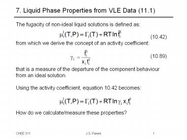
7. Liquid Phase Properties from VLE Data (11.1)
- The fugacity of non-ideal liquid solutions is
defined as - (10.42)
- from which we derive the concept of an activity
coefficient - (10.89)
- that is a measure of the departure of the
component behaviour from an ideal solution. - Using the activity coefficient, equation 10.42
becomes - How do we calculate/measure these properties?
2
Liquid Phase Properties from VLE Data
- Suppose we conduct VLE experiments on our system
of interest. - At a given temperature, we vary the system
pressure by changing the cell volume. - Wait until equilibrium is established (usually
hours) - Measure the compositions of the liquid and vapour
3
Liquid Solution Fugacity from VLE Data
- Our understanding of molecular dynamics does not
permit us to predict non-ideal solution fugacity,
fil . We must measure them by experiment, often
by studies of vapour-liquid equilibria. - Suppose we need liquid solution fugacity data for
a binary mixture of AB at P,T. At equilibrium, - The vapour mixture fugacity for component i is
given by, - (10.47)
- If we conduct VLE experiments at low pressure,
but at the required temperature, we can use the
perfect gas mixture model, - by assuming that ?iv 1.
4
Liquid Solution Fugacity from Low P VLE Data
- Since our experimental measurements are taken at
equilibrium, - according to the perfect gas
mixture model - What we need is VLE data at various pressures
(all relatively low)
5
Activity Coefficients from Low P VLE Data
- With a knowledge of the liquid solution fugacity,
we can derive activity coefficients. Actual
fugacity - Ideal solution fugacity
- Our low pressure vapour fugacity simplifies fil
to - and if P is close to Pisat
- leaving us with
6
Activity Coefficients from Low P VLE Data
- Our low pressure VLE data can now be processed to
yield experimental activity coefficient data
7
Activity Coefficients from Low P VLE Data
8
7. Correlation of Liquid Phase Data
- The complexity of molecular interactions in
non-ideal systems makes prediction of liquid
phase properties very difficult. - Experimentation on the system of interest at the
conditions (P,T,composition) of interest is
needed. - Previously, we discussed the use of low-pressure
VLE data for the calculation of liquid phase
activity coefficients. - As practicing engineers, you will rarely have the
time to conduct your own experiments. - You must rely on correlations of data developed
by other researchers. - These correlations are empirical models (with
limited fundamental basis) that reduce
experimental data to a mathematical equation. - In CHEE 311, we examine BOTH the development of
empirical models (thermodynamicists) and their
applications (engineering practice).
9
Correlation of Liquid Phase Data
- Recall our development of activity coefficients
on the basis of the partial excess Gibbs energy - where the partial molar Gibbs energy of the
non-ideal model is provided by equation 10.42 - and the ideal solution chemical potential is
- Leaving us with the partial excess Gibbs energy
- (10.90)
10
Correlation of Liquid Phase Data
- The partial excess Gibbs energy is defined by
- In terms of the activity coefficient,
- (10.94)
- Therefore, if as practicing engineers we have GE
as a function of P,T, xn (usually in the form of
a model equation) we can derive ?i. - Conversely, if thermodynamicists measure ?i, they
can calculate GE using the summability
relationship for partial properties. - (10.97)
- With this information, they can generate model
equations that practicing engineers apply
routinely.
11
Correlation of Liquid Phase Data
- We can now process this our MEK/toluene data one
step further to give the excess Gibbs energy, - GE/RT x1ln?1 x2ln?2
12
Correlation of Liquid Phase Data
- Note that GE/(RTx1x2) is reasonably represented
by a linear function of x1 for this system. This
is the foundation for correlating experimental
activity coefficient data
13
Correlation of Liquid Phase Data
- The chloroform/1,4-dioxane system exhibits a
negative deviation from Raoults Law. - This low pressure VLE data can be processed in
the same manner as the MEK/toluene system to
yield both activity coefficients and the excess
Gibbs energy of the overall system.
14
Correlation of Liquid Phase Data
- Note that in this example, the activity
coefficients are less than one, and the excess
Gibbs energy is negative. - In spite of the obvious difference from the
MEK/toluene system behaviour, the plot of
GE/x1x2RT is well approximated by a line.
15
8.4 Models for the Excess Gibbs Energy
- Models that represent the excess Gibbs energy
have several purposes - they reduce experimental data down to a few
parameters - they facilitate computerized calculation of
liquid phase properties by providing equations
from tabulated data - In some cases, we can use binary data (A-B, A-C,
B-C) to calculate the properties of
multi-component mixtures (A,B,C) - A series of GE equations is derived from the
Redlich/Kister expansion - Equations of this form fit excess Gibbs energy
data quite well. However, they are empirical and
cannot be generalized for multi-component (3)
mixtures or temperature.
16
Symmetric Equation for Binary Mixtures
- The simplest Redlich/Kister expansion results
from CD0 - To calculate activity coefficients, we express GE
in terms of moles n1 and n2. - And through differentiation,
- we find
17
7. Excess Gibbs Energy Models
- Practicing engineers find most of the
liquid-phase information needed for equilibrium
calculations in the form of excess Gibbs Energy
models. These models - reduce vast quantities of experimental data into
a few empirical parameters, - provide information an equation format that can
be used in thermodynamic simulation packages
(Provision) - Simple empirical models
- Symmetric, Margules, vanLaar
- No fundamental basis but easy to use
- Parameters apply to a given temperature, and the
models usually cannot be extended beyond binary
systems. - Local composition models
- Wilsons, NRTL, Uniquac
- Some fundamental basis
- Parameters are temperature dependent, and
multi-component behaviour can be predicted from
binary data.
18
Excess Gibbs Energy Models
- Our objectives are to learn how to fit Excess
Gibbs Energy models to experimental data, and to
learn how to use these models to calculate
activity coefficients.
19
Margules Equations
- While the simplest Redlich/Kister-type expansion
is the Symmetric Equation, a more accurate model
is the Margules expression - (11.7a)
- Note that as x1 goes to zero,
- and from Lhopitals rule we know
- therefore,
- and similarly
20
Margules Equations
- If you have Margules parameters, the activity
coefficients are easily derived from the excess
Gibbs energy expression - (11.7a)
- to yield
- (11.8ab)
- These empirical equations are widely used to
describe binary solutions. A knowledge of A12
and A21 at the given T is all we require to
calculate activity coefficients for a given
solution composition.
21
van Laar Equations
- Another two-parameter excess Gibbs energy model
is developed from an expansion of (RTx1x2)/GE
instead of GE/RTx1x2. The end results are - (11.13)
- for the excess Gibbs energy and
- (11.14)
- (11.15)
- for the activity coefficients.
- Note that as x1?0, ln?1? ? A12
- and as x2 ? 0, ln?2? ? A21
22
Local Composition Models
- Unfortunately, the previous approach cannot be
extended to systems of 3 or more components. For
these cases, local composition models are used to
represent multi-component systems. - Wilsons Theory
- Non-Random-Two-Liquid Theory (NRTL)
- Universal Quasichemical Theory (Uniquac)
- While more complex, these models have two
advantages - the model parameters are temperature dependent
- the activity coefficients of species in
multi-component liquids can be calculated from
binary data. - A,B,C A,B A,C B,C
- tertiary mixture binary binary binary
23
Wilsons Equations for Binary Solution Activity
- A versatile and reasonably accurate model of
excess Gibbs Energy was developed by Wilson in
1964. For a binary system, GE is provided by - (11.16)
- where
- (11.24)
- Vi is the molar volume at T of the pure
component i. - aij is determined from experimental data.
- The notation varies greatly between publications.
This includes, - a12 (?12 - ?11), a12 (?21 - ?22) that you
will encounter in Holmes, M.J. and M.V. Winkle
(1970) Ind. Eng. Chem. 62, 21-21.
24
Wilsons Equations for Binary Solution Activity
- Activity coefficients are derived from the excess
Gibbs energy using the definition of a partial
molar property - When applied to equation 11.16, we obtain
- (11.17)
- (11.18)
25
Wilsons Equations for Multi-Component Mixtures
- The strength of Wilsons approach resides in its
ability to describe multi-component (3) mixtures
using binary data. - Experimental data of the mixture of interest (ie.
acetone, ethanol, benzene) is not required - We only need data (or parameters) for
acetone-ethanol, acetone-benzene and
ethanol-benzene mixtures - The excess Gibbs energy is written
- (11.22)
- and the activity coefficients become
- (11.23)
- where ?ij 1 for ij. Summations are over all
species.
26
Wilsons Equations for 3-Component Mixtures
- For three component systems, activity
coefficients can be calculated from the following
relationship - Model coefficients are defined as (?ij 1 for
ij)
27
Comparison of Liquid Solution Models
Activity coefficients of 2-methyl-2-butene
n-methylpyrollidone. Comparison of experimental
values with those obtained from several equations
whose parameters are found from the
infinite-dilution activity coefficients. (1)
Experimental data. (2) Margules equation. (3)
van Laar equation. (4) Scatchard-Hamer equation.
(5) Wilson equation.