FIG. 1.1

1
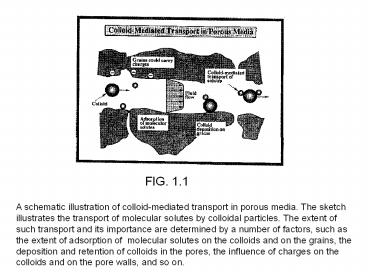
FIG. 1.1
A schematic illustration of colloid-mediated
transport in porous media. The sketch illustrates
the transport of molecular solutes by colloidal
particles. The extent of such transport and its
importance are determined by a number of factors,
such as the extent of adsorption of molecular
solutes on the colloids and on the grains, the
deposition and retention of colloids in the
pores, the influence of charges on the colloids
and on the pore walls, and so on.
2
FIG. 1.2
A simplified sketch of a hypothetical protein
molecule embedded in a bilayer (a biological
membrane ). The bilayer shown is a
two-dimensional cross section of a membrane. The
bundle of cylinders shown represents the
helices of a protein. The cylinders are part of
the same protein and are joined together by other
segments (not shown) of the protein protruding
out of the bilayer on either side.
3
TABLE 1.1
Some Exaples of Disciplines and Topics for which
Colloids and Colloidal Phenomena Are Important
4
Cut number Radius (cm) Number of spheres Volume per sphere(cm3) Area per sphere (cm2) Total area (cm2)
Original 1 1 4.19 1.26 101 1.26 101
Symbol Rs N0 V0 A0 AT,0
1 5 10-1 8 5.24 10-1 3.14 2.51 101
2 2.5 10-1 6.4 101 6.55 10-2 7.86 10-1 5.03 101
3 1.25 10-1 5.12 102 8.18 10-3 1.96 10-1 1.01 102
.
n (1/2)n Rs 8n N0 (1/8)nV0 (1/4)n A0 2n AT,0
.
19.93 10-6 1018 4.2 10-18 1.26 10-11 1.26 107
23.25 10-7 1021 4.2 10-21 1.26 10-13 1.26 108
26.58 10-8 1024 4.2 10-24 1.26 10-15 1.26 109
TABLE 1.2
The Radius, Area, and Volume per Particle, Number
of Particle, and Total Area for Any Array of
Spheres After n Cuts, Where a Cut is Defined to
Be the Reapportionment of Materials into
Particles With Radius that Is Half the Starting
Value
5
Cut number Radius (cm) Number of water molecules per sphere Number of water molecules at surface Fraction of total water molecules at surface Total surface energy(J)
0 1.0 1.38 1023 1.26 1015 9.13 10-8 9.07 10-5
1 5 10-1 1.75 1022 3.14 1015 1.79 10-7 1.81 10-4
2 2.5 10-1 2.18 1021 5.03 1016 3.64 10-7 3.62 10-4
3 1.25 10-1 2.73 1020 1.01 1017 7.32 10-7 7.27 10-4
. . . . . .
. . . . . .
19.93 10-6 1.4 105 1.26 1022 9.13 10-2 9.07 101
23.25 10-7 1.4 102 1.26 1023 9.13 10-1 9.07 102
26.58 10-8 1.4 10-1 1.26 1024 9.13 9.07 103
TABLE 1.3
Total Number of Water Molecules per Sphere and
Number at Surface for Spheres of Water After n
Cuts ( Also Total Surface Energy of the Array of
Spheres of Water
6
TABLE 1.4
Summary of Some of the Descriptive Names Used to
Designate Two-Phase Colloidal Systems
7
FIG. 1.3
Molecular cargo in a liposome. The cargo
molecules are carried in different parts of the
liposome depending on their chemical nature.
Hydrophobic molecules are carried inside the
hydrophobic part of the bilayer, whereas
hydrophilic molecules reside in the interior.
More complex molecules are wholly or partly
embedded in the bilayer or chemically bound to
the interior or exterior surface.
8
FIG. 1.4
A large-area, solid-state x-ray receptor with an
electrophoretic image display. When a voltage is
applied across the image cell, pigment particles
and counterions in the liquid separate. Most of
the voltage drop occurs across the Se layer.
X-ray exposure under this condition leads to the
creation of a charge-image at the
photoconductor-composite/liquid interface due to
the generation of x-ray-induced charges in the
Se. After the x-ray exposure, the applied voltage
is is reduced to zero, and the pigment particles
are driven to the viewing plate. The image become
visible on illumination
9
FIG. 1.5
Schematic illustration of kinetic stability of
colloids. The figure shows the interaction energy
(free energy) E as a function of the
surface-to-surface separation r between two
particles ( kb and T are the Boltzmann constant
and the absolute temperature of the dispersion ,
respectively ).(a) The free energy will reach the
global mininum if the two particles can come
close enough (r d). However , the energy
barrier against coagulation, ?Ec, is of the order
of the order of the thermal energy kBT, and
therefore the dispersion is kinetically unstable.
(b) The energy barrier ?EcgtgtkBT, and the
dispersion is kinetically stable since the
thermodynamically favored separation distance is
not reachable. ( See Chapters 11 and 13 for more
details.)
10
FIG. 1.6
A schematic diagram of colloidal processing of
ceramic specimens. The figure illustrates some of
the ways in which a dispersion is densified and
transformed into porous or compact films or bulk
objects. (Adapted and modified form Brinker and
Scherer 1990.)
11
FIG. 1.7
Some of the microstructures produced by the
self-association behavior of diblock copolymer
solution. The figure illustrates the (a)
spherical, (b) cylindrical, and (c) lamellar
structures (among other ) that are possible in
such solutions. Each diblock polymer chain
consists of strings of white beads ( representing
one type of homopolymer ) and strings of black
beads ( representing the second type of
homopolymer). (Redrawn form A. Yu. Grosberg and
A. Khokhlov, Statistical Physics of
Macromolecules, AIP Press, New York,1994.)
12
FIG. 1.8
Electron micrograph of cross-linked monodisperse
polystyrene latex particles. The latex is a
commercial product ( d 0.500 µm ) sold as a
calibration standard. (Photograph courtesy of
R.S.Daniel and L.X.Oakford, California State
Polytechnic University, Pomona,CA.
13
FIG. 1.9
Electron micrograph ( 150000 ) of carbon black
particles (a) before heat treatment and (b)
after heating to 2700? in the absence of
oxygen.(Adapted form F.A.Heckman, Rubber Chem.
Technol.37,1243(1964)
14
FIG. 1.10
Characterization of the size of irregular (a)
a schematic illustration of Martin diameters. (b)
the use of a graticule to estimate the
characteristic dimension.
15
FIG. 1.11
Ellipsoids of revolution (a) a prolate (a gt b )
ellipsoid and (b) an oblate ( a lt b ) ellipsoid
. The figure shows the relationship between the
semiaxes and the axis of revolution.
16
FIG. 1.12
Electron micrograph of two different types of
particles that represent extreme variations from
spherical particles (a) tobacco mosaic virus
particles ( Photograph courtesy of Carl Zeiss,
Inc., New York ) and (b), clay particles (
sodium kaplinite ) of mean diameter 0.2µm ( by
matching circular fields ). In both (a) and (b) ,
contrast has been enhanced by shadow casting (
see Section 1.6a.2a and Figure 1.21).(Adapted
form M.D.Luh and R.A.Bader,J.Colloid Interface
Sci.33,549(1997)
17
FIG. 1.13
Spherical and cubic model particles with
crystalline or amorphous microstructure (a)
spherical zinc sulfide particles ( transmission
electron microscopy , TEM , see Section 1.6a.2a)
x-ray diffraction studies show that the
microstructure of these particles is crystalline
(b) cubic lead sulfide particles ( scanning
electron microscopy, SEM, see Section 1.6a.2a)
(c) amorphous spherical particle of manganese(II)
phosphate (TEM) and (d) crystalline cubic
cadmium carbonate particles ( SEM ). (Reprinted
with permission of Matijevic 1993
18
FIG. 1.14
Model particles of different shapes with the
same or different chemical compositions (a)
rodlike particles of akageneite (ß-FeOOH )(b)
ellipsoidal particles of hematite (a-Fe2O3) (c)
cubic particles of hematite and (d) rodlike
particles of mixed chemical composition (a-Fe2O3
and ß-FeOOH ). All are TEM pictures.( Reprinted
with permission of Matijevic 1993.)
19
FIG. 1.15
Transmission electron micrographs of aggregates
of gold particles. These aggregates were made
from a gold colloid to study the relation between
the kinetics of aggregation and the resulting
structures of the aggregates ( see also Section
1.5b.2). The a-d portions of the illustration
show aggergates at various resolutions. ( The
pictures are not from the same aggregate.)
(Adapted from D.A. Weitz and J.S.Huang, in
kinetics of Aggregation and Gelation, F.Family
and D.O.Landau, Eds.,Elsevier, Amsterdam,
Netherlands, 1984.)
20
FIG. 1.16
The total area measured versus the diameter of
the aggregate on a log-log scale for the data
given in Example 1.2.
21
FIG. 1.17
Aggregates obtained through computer simulations
using various growth models. The figure shows
typical aggregates produced in the simulations
under a number of conditions. The results show
two-dimensional renditions of three-dimensional
simulations. The column headings identify the
controlling step in the aggregation process
(i.e., the type of particle motion and
probability of adhesion pa). (reaction limited
implies pa 1 ballistic implies that the
particle motion is rectilinear with the added
assumption that pa 1 diffusion limited
implies that the pareiclemotion is a random
walk with the assumption that pa 1.) The
row labels specify which type of collision is
considered (i.e., monomer-cluster or
cluster-cluster ). The names associated with the
models are also shown. For example,
diffusion-limited monomer-cluster aggregation
(DLMCA) is known as the Witten-Sander model.
(RLCCA signifies reaction-limited cluster-cluster
aggregation.) (Redrawn from D.W.Schaefer, MRS
Bulletin 8,22 (1988). Simulation are from P.
Meakin, in On Growth and Form, H.E.Stanley and N.
Ostrowsky, Eds., Martinus-Nijhoff, Boston, 1986.)
22
TABLE 1.5
A Hypothetical Distribution of 400 Spherical
particles
23
FIG. 1.18
Graphical representation of data in Table1.5.
Data are presented as (a) a histogram and (b) a
cumulative distribution curve.
24
TABLE 1.6
Some of the More Widely Encountered Size
Averages in Surface and Colloid Science
25
TABLE 1.7
Number of Moles and Molecular Weights for Eight
Classes of a Hypothetical Fractionated Polymer (
Remaining Quantities Calculated in Example 1.3)
26
TABLE 1.8
The Most Common Molecular Weight Averages, Their
Definitions, and Their Methods of Determination
27
FIG. 1.19
Basic optical principle governing the operation
of an optical microscope (a) the geometry on
which the resolving power d of a microscope is
based (b) detail showing how light from both
sources must be intercepted by the lens become
part of the image.
28
FIG. 1.20
Schematic comparision of (a) light and (b)
electron microscopes showing components that
perform parallel functions in eath.
29
FIG. 1.21
Shadowing of a spherical particle using metal
vapor (a) side view and (b) top view.
30
FIG. 1.22
One type of operation of a scanning tunneling
microscope (STM). A tunneling current I flows
between the sharp tip of the probe and surface
when a bias voltage V is applied to the sample. A
computer monitors the tunneling current and
adjusts the distance between the probe and the
surface such that a constant tunneling current
Iref is maintained. The resulting changes in the
position of the tip are then recorded and
converted to an image such as the one shown on
the monitor or the one shown in the inset. The
image shown in the inset is that of an atomically
smooth nickel surface. The periodic arrangement
of the atoms on the surface can be seen clearly
in the STM image.
31
FIG. 1.23
Plot of log M and detector output versus
retention volume for size-exclusion
chromatography. Also shown is the relation among
VR, VV, VP, and KiVp as discussed in the text.
32
FIG. 1.24
Size exclusion of a particle in a pore (a)
exclusion of a spherical particle in a
cylindrical pore and (b) exclusion of
macromolecules. Particles shown in dashed lines
indicate positions or orientations that are
excluded.
33
FIG. 1.25
Shape selectivity of a zeolite cage. The cage
allows (a) straight-chain hydrocarbons to snake
their way into the pores while (b) preventing
branched-chain hydrocarbons from entry.
34
FIG. 1.26
Examples of various types of measurements that
provide information on the forces between
particles and surfaces (a) adhesion
measurements (b) peeling measurements (c)
contact angle measurements (see Chapter 6 ) (d)
equilibrium thickness of thin free films (e)
equilibrium thickness of thin adsorbed films
(examples of practical applications include
wetting of hydrophilic surfaces by water,
adsorption of molecules from vapor, protective
surface coatings and lubricatant layers,
photographic films see Chapters 6 and 9) (f)
interparticle spacing in liquids ( examples of
applications include colloidal suspensions,
paints, pharmaceutical dispersion see
Chapter13) (g)sheetlike particle spacings in
liquids ( examples of practical applications
include clay and soil-swelling behavior,
microstructure of soaps and biological
membranes)(h) coagulation studies
35
FIG. 1.27 (a)
36
FIG. 1.27 (b)
Continued