
HASHING - PowerPoint PPT Presentation
Title: HASHING
1
HASHING
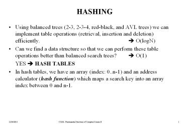
- Using balanced trees (2-3, 2-3-4, red-black, and
AVL trees) we can implement table operations
(retrieval, insertion and deletion)
efficiently. ? O(logN) - Can we find a data structure so that we can
perform these table operations better than
balanced search trees? ? O(1) - YES ? HASH TABLES
- In hash tables, we have an array (index 0..n-1)
and an address calculator (hash function) which
maps a search key into an array index between 0
and n-1.
2
Hash Function Address Calculator
Hash Function
Hash Table
3
Hashing
- A hash function tells us where to place an item
in array called a hash table. This method is
know as hashing. - A hash function maps a search key into an integer
between 0 and n-1. - We can have different hash functions.
- Ex. h(x) x mod n if x is an integer
- The hash function is designed for the search keys
depending on the data types of these search keys
(int, string, ...) - Collisions occur when the hash function maps more
than one item into the same array. - We have to resolve these collisions using certain
mechanism. - A perfect hash function maps each search key into
a unique location of the hash table. - A perfect hash function is possible if we know
all the search keys in advance. - In practice (we do not know all the search keys),
a hash function can map more than one key into
the same location (collision).
4
Hash Function
- We can design different hash functions.
- But a good hash function should
- be easy and fast to compute,
- place items evenly throughout the hash table.
- We will consider only hash functions operate on
integers. - If the key is not an integer, we map it into an
integer first, and apply the hash function. - The hash table size should be prime.
- By selecting the table size as a prime number, we
may place items evenly throughout the hash table,
and we may reduce the number of collisions.
5
Hash Functions -- Selecting Digits
- If the search keys are big integers (Ex.
nine-digit numbers), we can select certain digits
and combine to create the address. - h(033475678) 37 selecting 2nd and 5th
digits (table size is 100) - h(023455678) 25
- Digit-Selection is not a good hash function
because it does not place items evenly throughout
the hash table.
6
Hash Functions Folding
- Folding Selecting all digits and add them
- h(033475678) 0 3 3 4 7 5 6 7 8
43 - 0 ? h(nine-digit search key) ? 81
- We can select a group of digits and we can add
these groups too.
7
Hash Functions Modula Arithmetic
- Modula arithmetic provides a simple and effective
hash function. - We will use modula arithmetic as our hash
function in the rest of our discussions. - h(x) x mod tableSize
- The table size should be prime.
- Some prime numbers 7,11, 13, ..., 101, ...
8
Hash Functions Converting Character String into
An Integer
- If our search keys are strings, first we have to
convert the string into an integer, and apply a
hash function which is designed to operate on
integers to this integer value to compute the
address. - We can use ASCII codes of characters in the
conversion. - Consider the string NOTE, assign 1 (00001) to
A, .... - N is 14 (01110), O is 15 (01111), T is 20
(10100), E is 5 ((00101) - Concatenate four binary numbers to get a new
binary number - 011100111111010000101 ? 474,757
- apply x mod tableSize
9
Collision Resolution
- There are two general approaches to collision
resolution in hash tables - Open Addressing Each entry holds one item
- Chaining Each entry can hold more than item
- Buckets hold certain number of items
10
A Collision
- Table size is 101
11
Open Addressing
- During an attempt to insert a new item into a
table, if the hash function indicates a location
in the hash table that is already occupied, we
probe for some other empty (or open) location in
which to place the item.The sequence of locations
that we examine is called the probe sequence. - ? If a scheme which uses this approach we say
that - it uses open addressing
- There are different open-addressing schemes
- Linear Probing
- Quadratic Probing
- Double Hashing
12
Open Addressing Linear Probing
- In linear probing, we search the hash table
sequentially starting from the original hash
location. - If a location is occupied, we check the next
location - We wrap around from the last table location to
the first table location if necessary.
13
Linear Probing - Example
- Example
- Table Size is 11 (0..10)
- Hash Function h(x) x mod 11
- Insert keys
- 20 mod 11 9
- 30 mod 11 8
- 2 mod 11 2
- 13 mod 11 2 ? 213
- 25 mod 11 3 ? 314
- 24 mod 11 2 ? 21, 22, 235
- 10 mod 11 10
- 9 mod 11 9 ? 91, 92 mod 11 0
0 9
1
2 2
3 13
4 25
5 24
6
7
8 30
9 20
10 10
14
Linear Probing Clustering Problem
- One of the problems with linear probing is that
table items tend to cluster together in the hash
table. - This means that the table contains groups of
consecutively occupied locations. - This phenomenon is called primary clustering.
- Clusters can get close to one another, and merge
into a larger cluster. - Thus, the one part of the table might be quite
dense, even though another part has relatively
few items. - Primary clustering causes long probe searches and
therefore decreases the overall efficiency.
15
Open Addressing Quadratic Probing
- Primary clustering problem can be almost
eliminated if we use quadratic probing scheme. - In quadratic probing,
- We start from the original hash location i
- If a location is occupied, we check the locations
i12 , i22 , i32 , i42 ... - We wrap around from the last table location to
the first table location if necessary.
16
Quadratic Probing - Example
- Example
- Table Size is 11 (0..10)
- Hash Function h(x) x mod 11
- Insert keys
- 20 mod 11 9
- 30 mod 11 8
- 2 mod 11 2
- 13 mod 11 2 ? 2123
- 25 mod 11 3 ? 3124
- 24 mod 11 2 ? 212, 2226
- 10 mod 11 10
- 9 mod 11 9 ? 912, 922 mod 11,
- 932 mod 11 7
0
1
2 2
3 13
4 25
5
6 24
7 9
8 30
9 20
10 10
17
Open Addressing Double Hashing
- Double hashing also reduces clustering.
- In linear probing and and quadratic probing , the
probe sequences are independent from the key. - We can select increments used during probing
using a second hash function. The second hash
function h2 should be - h2(key) ? 0
- h2 ? h1
- We first probe the location h1(key)
- If the location is occupied, we probe the
location h1(key)h2(key), h1(key)(2h2(key)),
...
18
Double Hashing - Example
- Example
- Table Size is 11 (0..10)
- Hash Function h1(x) x mod 11
- h2(x) 7 (x mod 7)
- Insert keys
- 58 mod 11 3
- 14 mod 11 3 ? 3710
- 91 mod 11 3 ? 37, 327 mod 116
0
1
2
3 58
4
5
6 91
7
8
9
10 14
19
Open Addressing Retrieval Deletion
- In open addressing, to find an item with a given
key - We probe the locations (same as insertion) until
we find the desired item or we reach to an empty
location. - Deletions in open addressing cause complications
- We CANNOT simply delete an item from the hash
table because this new empty (deleted locations)
cause to stop prematurely (incorrectly)
indicating a failure during a retrieval. - Solution We have to have three kinds of
locations in a hash table Occupied, Empty,
Deleted. - A deleted location will be treated as an occupied
location during retrieval and insertion.
20
Separate Chaining
- Another way to resolve collisions is to change
the structure of the hash table. - In open-addressing, each location of the hash
table holds only one item. - We can define a hash table so that each location
is itself an array called bucket, we can store
the items which hash into this location in this
array. - Problem What will be the size of the bucket?
- A better approach is to design the hash table as
an array of linked lists, this collision
resolution method is known as separate-chaining. - In separate-chaining , each entry (of the hash
table) is a pointer to a linked list (the chain)
of the items that the hash function has mapped
into that location.
21
Separate Chaining
22
Hashing - Analysis
- An analysis of the average-case efficiency of
hashing involves the load factor ?, which is
the ration of the current number of items in
the table to the table size. - ? (current number of items) / tableSize
- The load factor measures how full a hash table
is. - The hash table should be so filled too much to
get better performance from the hashing. - Unsuccessful searches generally require more time
than successful searches. - In average case analyses, we assume that the hash
function uniformly distributes the keys in the
hash table.
23
Linear Probing Analysis
- For linear probing, the approximate average
number of comparisons (probes) that a search
requires as follows
for a successful search
for an unsuccessful search
- As load factor increases, the number of
collisions increases - causing increased search times.
- To maintain efficiency, it is important to
prevent the hash table - from filling up.
24
Linear Probing Analysis -- Example
- What is the average number of probes for a
successful search and an unsuccessful search for
this hash table? - Hash Function h(x) x mod 11
- Successful Search
- 20 9 -- 30 8 -- 2 2 -- 13 2, 3 --
25 3,4 - 24 2,3,4,5 -- 10 10 -- 9 9,10, 0
- Avg. Probe for SS (11122413)/815/8
- Unsuccessful Search
- We assume that the hash function uniformly
distributes the keys. - 0 0,1 -- 1 1 -- 2 2,3,4,5,6 -- 3
3,4,5,6 - 4 4,5,6 -- 5 5,6 -- 6 6 -- 7 7 -- 8
8,9,10,0,1 - 9 9,10,0,1 -- 10 10,0,1
- Avg. Probe for US
- (21543211543)/1131/11
0 9
1
2 2
3 13
4 25
5 24
6
7
8 30
9 20
10 10
25
Quadratic Probing Double Hashing Analysis
- For quadratic probing and double hashing, the
approximate average number of comparisons
(probes) that a search requires as follows
for a successful search
for an unsuccessful search
- On average, both methods require fewer
comparisons than - linear probing.
26
Separate Chaining
- For separate-chaining, the approximate average
number of comparisons (probes) that a search
requires as follows
for a successful search
for an unsuccessful search
- Separate-chaining is most efficient collision
resolution scheme. - But it requires more storage. We need storage
for the pointer fields. - We can easily perform deletion operation using
separate-chaining - scheme. Deletion is very difficult in
open-addressing.
27
The relative efficiency of four
collision-resolution methods
28
What Constitutes a Good Hash Function
- A hash function should be easy and fast to
compute. - A hash function should scatter the data evenly
throughout the hash table. - How well does the hash function scatter random
data? - How well does the hash function scatter
non-random data? - Two general principles
- The hash function should use entire key in the
calculation. - If a hash function uses modulo arithmetic, the
table size should be prime.
29
Hash Table versus Search Trees
- In the most of operations, the hash table
performs better than search trees. - But, the traversing the data in the hash table in
a sorted order is very difficult. - For similar operations, the hash table will not
be good choice. - Ex. Finding all the items in a certain range.
30
Data with Multiple Organizations
- Several independent data structure do not support
all operations efficiently. - We may need multiple organizations for data to
get efficient implementations for all operations. - One organization will be used for certain
operations, the other organizations will be used
for other operations.
31
Data with Multiple Organizations (cont.)
32
Data with Multiple Organizations (cont.)
Recommended
CrystalGraphics Presentations


