
Raw H2RG Image - PowerPoint PPT Presentation
Title:
Raw H2RG Image
Description:
Raw H2RG Image Two Hawaii2RG images provided by Gert Finger is the starting point of this analysis of the nosie variance in the images, normally use for the Photon ... – PowerPoint PPT presentation
Number of Views:37
Avg rating:3.0/5.0
Title: Raw H2RG Image
1
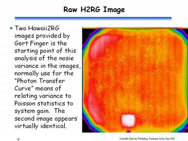
Raw H2RG Image
- Two Hawaii2RG images provided by Gert Finger is
the starting point of this analysis of the nosie
variance in the images, normally use for the
Photon Transfer Curve means of relating
variance to Poisson statistics to system gain.
The second image appears virtually identical.
2
Difference H2RG image
- The difference of these two images still shows
structure, but much of it has disappeared. Note
the vertical stripes which will appear
prominently in the power spectrum.
3
Central 1024 Difference
- Choosing the central 1024x1024 pixels in
preparation for Fourier transforming the
difference. - Again, note not only the wide-spaced vertial
stripes, but the closely spaced stripes.
4
Power Spectrum
- The power spectrum of the difference shows noise
which has obvious power features - Horizontal line vertical stripes
- Spots closely spaced vertical stripes
- Central spot various large-scale features
remaining in difference
5
Binned Power Spectrum
- Binning the power spectrum 8x8 and increasing the
stretch makes non-uniformity in the power
spectrum more obvious. - The power at the Nyquist frequency (corners) is
significantly smaller than the asymptote as k -gt
0. - The Poisson variance from the photons impinging
on the detector has been suppressed by
convolution with some sort of pixel-to-pixel
correlation. The best estimate of the
pre-convolution is the k-gt0 asymptote. - There is also significant non-circular uniformity
apparent, indicating that the convolution is
worse in the horizontal direction than the
vertical direction.
6
Masked for Averaging
- To make a quantitative estimate of the error in
variance estimation, mask out the features which
are obviously caused by large scale detector
characteristics rather than pixel-to-pixel
correlations.
7
Azimuthal Average
- Despite the fact that the power spectrum is not
accurately circular, take an azimuthal average so
that we can examine the power spectrum as a
function of k.
8
Power Spectrum as a function of k
- Take a cut through the azimuthal average to show
the variance as a function of wavenumber. - The big peak at k0 is large-scale structure
which is caused by detector non-uniformities. - K63 is the Nyquist frequency and the direct
pixel-to-pixel correlation. - The big challenge is to understand what variance
comes from pixel-to-pixel variations and what
comes from large scale structure. We have used
differencing to suppress the latter, but it is
not perfect.
9
Ln Power Spectrum and k2 Fit
- As a naïve starting point, imagine that the
pixel-to-pixel correlation has a Gaussian form.
If so we can fit the natural log of the power
with a parabola. - This has a reasonable match to high k, but
obviously does not explain low k large-scale
features.
10
Ln Power Spectrum and k4 Fit
11
Ln Power Spectrum and k4 Fit
- A more likely pixel-to-pixel correlation arises
from mutual capacitance, which might vary as r-3.
I dont recall the 2-D Fourier tranform of this,
but a Lorenzian FTs to an exponential, so we
might expect that ln power should go linearly
with k. Fitting a quartic polynomial
demonstrates another division of power between
pixel-to-pixel variance and large scale detector
structure. - Quantitatively, the difference between Nyquist
and k0 is an offset in logarithm of 0.20, which
means that a gain determined by variance over
signal will be underestimated by a factor of
1.22.
Recommended
CrystalGraphics Presentations


