Variable-Frequency Response Analysis

1
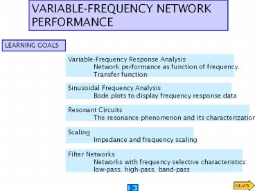
VARIABLE-FREQUENCY NETWORK PERFORMANCE
LEARNING GOALS
Variable-Frequency Response Analysis Network
performance as function of frequency. Transfer
function
Sinusoidal Frequency Analysis Bode plots to
display frequency response data
Resonant Circuits The resonance phenomenon and
its characterization
Scaling Impedance and frequency scaling
Filter Networks Networks with frequency
selective characteristics low-pass, high-pass,
band-pass
2
VARIABLE FREQUENCY-RESPONSE ANALYSIS
In AC steady state analysis the frequency is
assumed constant (e.g., 60Hz). Here we consider
the frequency as a variable and examine how the
performance varies with the frequency.
Variation in impedance of basic components
3
(No Transcript)
4
(No Transcript)
5
Frequency dependent behavior of series RLC network
6
Simplified notation for basic components
Moreover, if the circuit elements (L,R,C,
dependent sources) are real then the expression
for any voltage or current will also be a
rational function in s
MATLAB can be effectively used to compute
frequency response characteristics
7
USING MATLAB TO COMPUTE MAGNITUDE AND PHASE
INFORMATION
NOTE Instead of comma (,) one can use space
to separate numbers in the array
num152.531e-3,0 den0.12.531e-3,152.
531e-3,1 freqs(num,den)
8
GRAPHIC OUTPUT PRODUCED BY MATLAB
Log-log plot
Semi-log plot
9
LEARNING EXAMPLE
A possible stereo amplifier
Desired frequency characteristic (flat between
50Hz and 15KHz)
Log frequency scale
Postulated amplifier
10
Frequency Analysis of Amplifier
Frequency dependent behavior is caused by
reactive elements
11
Some nomenclature
NETWORK FUNCTIONS
When voltages and currents are defined at
different terminal pairs we define the ratios as
Transfer Functions
If voltage and current are defined at the same
terminals we define Driving Point
Impedance/Admittance
To compute the transfer functions one must
solve the circuit. Any valid technique is
acceptable
12
The textbook uses mesh analysis. We will use
Thevenins theorem
13
(More nomenclature)
POLES AND ZEROS
Arbitrary network function
Using the roots, every (monic) polynomial can be
expressed as a product of first order terms
The network function is uniquely determined by
its poles and zeros and its value at some other
value of s (to compute the gain)
14
LEARNING EXTENSION
Find the driving point impedance at
Replace numerical values
15
LEARNING EXTENSION
16
SINUSOIDAL FREQUENCY ANALYSIS
Circuit represented by network function
17
HISTORY OF THE DECIBEL
Originated as a measure of relative (radio) power
Using log scales the frequency characteristics of
network functions have simple asymptotic
behavior. The asymptotes can be used as
reasonable and efficient approximations
18
General form of a network function showing basic
terms
Display each basic term separately and add
the results to obtain final answer
Lets examine each basic term
19
Constant Term
Poles/Zeros at the origin
20
Behavior in the neighborhood of the corner
Low freq. Asym.
21
Simple zero
Simple pole
22
Quadratic pole or zero
Corner/break frequency
Resonance frequency
These graphs are inverted for a zero
23
Generate magnitude and phase plots
LEARNING EXAMPLE
Draw asymptotes for each term
Draw composites
24
asymptotes
25
Generate magnitude and phase plots
LEARNING EXAMPLE
Draw asymptotes for each
Form composites
26
Final results . . . And an extra hint on poles at
the origin
27
Sketch the magnitude characteristic
LEARNING EXTENSION
We need to show about 4 decades
Put in standard form
28
Sketch the magnitude characteristic
LEARNING EXTENSION
Once each term is drawn we form the composites
29
Sketch the magnitude characteristic
LEARNING EXTENSION
Put in standard form
Once each term is drawn we form the composites
30
LEARNING EXAMPLE
A function with complex conjugate poles
Put in standard form
Draw composite asymptote
Behavior close to corner of conjugate
pole/zero is too dependent on damping
ratio. Computer evaluation is better
31
Evaluation of frequency response using MATLAB
Using default options
num25,0 define numerator polynomial
denconv(1,0.5,1,4,100) use CONV for
polynomial multiplication den 1.0000
4.5000 102.0000 50.0000 freqs(num,den)
32
Evaluation of frequency response using MATLAB
User controlled
gtgt clear all close all clear workspace and
close any open figure
gtgt figure(1) open one figure window (not
STRICTLY necessary)
gtgt wlogspace(-1,3,200)define x-axis, 10-1
- 103, 200pts total
gtgt G25jw./((jw0.5).((jw).24jw100))
compute transfer function
gtgt subplot(211) divide figure in two. This is
top part gtgt semilogx(w,20log10(abs(G))) put
magnitude here
gtgt grid put a grid and give proper title and
labels gtgt ylabel('G(j\omega)(dB)'), title('Bode
Plot Magnitude response')
33
Evaluation of frequency response using MATLAB
User controlled
Continued
USE TO ZOOM IN A SPECIFIC REGION OF INTEREST
Repeat for phase
gtgt semilogx(w,unwrap(angle(G)180/pi)) unwrap
avoids jumps from 180 to -180 gtgt grid,
ylabel('Angle H(j\omega)(\circ)'), xlabel('\omega
(rad/s)')
gtgt title('Bode Plot Phase Response')
No xlabel here to avoid clutter
34
LEARNING EXTENSION
Sketch the magnitude characteristic
35
num0.21,1 denconv(1,0,1/144,1/36,1)
freqs(num,den)
36
DETERMINING THE TRANSFER FUNCTION FROM THE BODE
PLOT
This is the inverse problem of determining
frequency characteristics. We will use only the
composite asymptotes plot of the magnitude to
postulate a transfer function. The slopes will
provide information on the order
A. different from 0dB. There is a constant Ko
B. Simple pole at 0.1
C. Simple zero at 0.5
D. Simple pole at 3
E. Simple pole at 20
If the slope is -40dB we assume double real pole.
Unless we are given more data
37
Determine a transfer function from the composite
magnitude asymptotes plot
LEARNING EXTENSION
A. Pole at the origin. Crosses 0dB line at 5
B. Zero at 5
D
C. Pole at 20
D. Zero at 50
E. Pole at 100
38
RESONANT CIRCUITS - SERIES RESONANCE
39
RESONANT CIRCUITS
These are circuits with very special frequency
characteristics And resonance is a very
important physical phenomenon
The frequency at which the circuit becomes purely
resistive is called the resonance frequency
40
Properties of resonant circuits
At resonance the impedance/admittance is minimal
Current through the serial circuit/ voltage
across the parallel circuit can become very large
(if resistance is small)
Given the similarities between series and
parallel resonant circuits, we will focus on
serial circuits
41
Properties of resonant circuits
At resonance the power factor is unity
42
Determine the resonant frequency, the voltage
across each element at resonance and the value of
the quality factor
LEARNING EXAMPLE
43
Given L 0.02H with a Q factor of 200, determine
the capacitor necessary to form a circuit
resonant at 1000Hz
LEARNING EXAMPLE
What is the rating for the capacitor if the
circuit is tested with a 10V supply?
The reactive power on the capacitor exceeds 12kVA
44
LEARNING EXTENSION
Find the value of C that will place the circuit
in resonance at 1800rad/sec
Find the Q for the network and the magnitude of
the voltage across the capacitor
45
Resonance for the series circuit
46
The Q factor
Q can also be interpreted from an energy point of
view
47
ENERGY TRANSFER IN RESONANT CIRCUITS
48
LEARNING EXAMPLE
Determine the resonant frequency, quality factor
and bandwidth when R2 and when R0.2
49
A series RLC circuit as the following properties
LEARNING EXTENSION
Determine the values of L,C.
1. Given resonant frequency and bandwidth
determine Q. 2. Given R, resonant frequency and Q
determine L, C.
50
LEARNING EXAMPLE
Find R, L, C so that the circuit operates as a
band-pass filter with center frequency of
1000rad/s and bandwidth of 100rad/s
Strategy 1. Determine Q 2. Use value of
resonant frequency and Q to set up two equations
in the three unknowns 3. Assign a value to
one of the unknowns
51
PROPERTIES OF RESONANT CIRCUITS VOLTAGE ACROSS
CAPACITOR
But this is NOT the maximum value for the voltage
across the capacitor
52
LEARNING EXAMPLE
Natural frequency depends only on L, C. Resonant
frequency depends on Q.
Using MATLAB one can display the frequency
response
53
R50 Low Q Poor selectivity
R1 High Q Good selectivity
54
The Tacoma Narrows Bridge
LEARNING EXAMPLE
Opened July 1, 1940 Collapsed Nov 7, 1940
Likely cause wind varying at frequency similar
to bridge natural frequency
55
Tacoma Narrows Bridge Simulator
Assume a low Q2.39
56
PARALLEL RLC RESONANT CIRCUITS
Impedance of series RLC
Admittance of parallel RLC
57
VARIATION OF IMPEDANCE AND PHASOR DIAGRAM
PARALLEL CIRCUIT
58
If the source operates at the resonant frequency
of the network, compute all the branch currents
LEARNING EXAMPLE
59
LEARNING EXAMPLE
60
LEARNING EXAMPLE
Increasing selectivity by cascading low Q circuits
Single stage tuned amplifier
61
Determine the resonant frequency, Q factor and
bandwidth
LEARNING EXTENSION
62
LEARNING EXTENSION
63
The resistance of the inductor coils cannot
be neglected
PRACTICAL RESONANT CIRCUIT
How do you define a quality factor for this
circuit?
64
LEARNING EXAMPLE
65
RESONANCE IN A MORE GENERAL VIEW
For series connection the impedance reaches
maximum at resonance. For parallel connection the
impedance reaches maximum
A high Q circuit is highly under damped
66
SCALING
Scaling techniques are used to change an
idealized network into a more realistic one or
to adjust the values of the components
Magnitude scaling does not change the frequency
characteristics nor the quality of the network.
67
LEARNING EXAMPLE
Determine the value of the elements and the
characterisitcs of the network if the circuit is
magnitude scaled by 100 and frequency scaled by
1,000,000
68
LEARNING EXTENSION
69
FILTER NETWORKS
Networks designed to have frequency selective
behavior
COMMON FILTERS
We focus first on PASSIVE filters
70
Simple low-pass filter
71
Simple high-pass filter
72
Simple band-pass filter
73
Simple band-reject filter
74
LEARNING EXAMPLE
Depending on where the output is taken, this
circuit can produce low-pass, high-pass or
band-pass or band- reject filters
High-pass
Low-pass
75
LEARNING EXAMPLE
A simple notch filter to eliminate 60Hz
interference
76
LEARNING EXTENSION
77
LEARNING EXTENSION
78
LEARNING EXTENSION
Band-pass
79
ACTIVE FILTERS
Passive filters have several limitations
1. Cannot generate gains greater than one
2. Loading effect makes them difficult to
interconnect
3. Use of inductance makes them difficult to
handle
Using operational amplifiers one can design all
basic filters, and more, with only resistors and
capacitors
The linear models developed for operational
amplifiers circuits are valid, in a more general
framework, if one replaces the resistors by
impedances
80
Basic Inverting Amplifier
81
Basic Non-inverting amplifier
Due to the internal op-amp circuitry, it
has limitations, e.g., for high frequency
and/or low voltage situations. The
Operational Transductance Amplifier (OTA)
performs well in those situations
82
Operational Transductance Amplifier (OTA)
COMPARISON BETWEEN OP-AMPS AND OTAs PHYSICAL
CONSTRUCTION
83
(No Transcript)
84
Basic OTA Circuits
85
OTA APPLICATION
Basic OTA Adder
86
(No Transcript)
87
LEARNING EXAMPLE
88
LEARNING EXAMPLE
Floating simulated resistor
The resistor cannot be produced with this OTA!
89
LEARNING EXAMPLE
Case b
Reverse polarity of v2!
Two equations in three unknowns. Select one
transductance
90
ANALOG MULTIPLIER
Based on modulating the control current
91
AUTOMATIC GAIN CONTROL
For simplicity of analysis we drop the absolute
value
92
OTA-C CIRCUITS
Circuits created using capacitors, simulated
resistors, adders and integrators
Frequency domain analysis assuming ideal OTAs
93
LEARNING EXAMPLE
Two equations in three unknowns. Select the
capacitor value
94
TOW-THOMAS OTA-C BIQUAD FILTER
95
LEARNING EXAMPLE
96
Bode plots for resulting amplifier
97
Using a low-pass filter to reduce 60Hz ripple
LEARNING BY APPLICATION
Design criterion place the corner frequency at
least a decade lower
98
Filtered output
99
LEARNING EXAMPLE
Single stage tuned transistor amplifier
Select the capacitor for maximum gain at 91.1MHz
Transistor
Parallel resonant circuit
100
LEARNING BY DESIGN
Anti-aliasing filter
Nyquist Criterion When digitizing an analog
signal, such as music, any frequency
components greater than half the sampling rate
will be distorted
In fact they may appear as spurious components.
The phenomenon is known as aliasing.
SOLUTION Filter the signal before digitizing,
and remove all components higher than half the
sampling rate. Such a filter is an anti-aliasing
filter
For CD recording the industry standard is to
sample at 44.1kHz. An anti-aliasing filter will
be a low-pass with cutoff frequency of 22.05kHz
101
Two-stage buffered filter
Improved anti-aliasing filter
102
LEARNING BY DESIGN
Notch filter to eliminate 60Hz hum
To design, pick one, e.g., C and determine the
other
103
ANTI ALIASING FILTER FOR MIXED MODE CIRCUITS
DESIGN EXAMPLE
Signals of different frequency and the
same samples
Visualization of aliasing
Ideally one wants to eliminate frequency
components higher than twice the sampling
frequency and make sure that all useful
frequencies as properly sampled
104
DESIGN EXAMPLE
BASS-BOOST AMPLIFIER
DESIRED BODE PLOT
105
DESIGN EXAMPLE
TREBLE BOOST
Original player response
Desired boost