Linear regression and linear modelling

1
Linear regression and linear modelling
2
Height and Weight
3
Height and Weight
4
Height and Weight
5
Height and Weight
6
Data exploration and Statistical analysis

1. Data checking, identifying problems and
   characteristics
2. Understanding chance and uncertainty
3. How will the data for one attribute behave, in a
   theoretical framework?
4. Theoretical framework assumes complete
   information, need to address uncertainties in
   real data
5. Testing your beliefs, do the data support what
   you think is true?
6. What happens when the assumptions of the
   theoretical framework are not valid
7. Modeling relationships between multiple outcomes
   and a numerical response

7
Data
8
Height and Weight
9
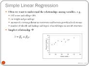
Simple linear regression

• Apparently linear relation, can we quantify this
  relation?
• Statistical modelling describing the
  relationship between height and weight with a
  straight line equation
• y is dependent on x, and therefore refer to y as
  the dependent variable or the response x is the
  explanatory variable.
• ? is the error, assumed to be 0 on average.

10
Mathematics of linear regression
11
Mathematics of linear regression
12
Simple linear regression

• Main goal is to find ? and ?, in the presence of
  uncertainty given the data
• Case Study

13
Simple Linear Regression

• Research Questions
• Can we determine the relationship between pH and
  time after slaughter? (Yes)
• If yes, can we quantify the relationship? (Yes)
  
• Can we predict pH given the time of slaughter?
  (Yes and no)

14
Extrapolation of Data

• Often convenient to extrapolate result to data
  outside range of regression, and just as often
  erroneous.
• In the meat processing example
• Will not expect the pH level to carry on
  decreasing with time, otherwise mathematically
  possible to attain zero or even negative pH, with
  sufficiently long duration.
• More logical to expect pH level to taper off to a
  stable level.

Dangerous to extrapolate results beyond range of
regression!
15
Interpreting Coefficients

• ?0 is the mean response when x 0
• ?1 is the change in y when x changes by one unit
• e.g. In the meat processing example
• ?0 is the average pH level when log(time) 0, or
  after one hour of slaughter.
• ?1 is the expected difference in pH between two
  steers whose log(time) differs by one unit.

16
Statistical inference in linear regression

• Test the significance (or contribution) of an
  independent variable (x) to the dependent
  variable (y) via hypothesis tests (or confidence
  intervals).
• Consider null hypothesis of H0 ? 0
• Tests linear relationship using t-tests.
• Often performed by default by softwares in
  regression.

17
Statistical inference in linear regression
In SPSS (for the meat processing example)
p-value lt 0.0001
tobs -0.726 / 0.034 - 21.08
18
Confidence bands

• Regression equation effectively provides a
  spectrum of estimated values
• In statistics, always quantify the uncertainty
  involved in estimation.
• Can construct confidence interval for every
  point along the line.
• Result is a confidence band.

19
Confidence Bands
20
Multiple regression and linear modelling

• More than one explanatory variable, example age,
  gender, ethnic groups and height
• Interested to find how these variables affect
  weight.
• Mathematically complicated, but conceptually
  identical to finding the coefficients which
  minimises the errors (easy with a computer)
• Notice the difference for categorical variables
  like gender and smoke. I(?) represents an
  indicator variable, taking the value 1 when the
  condition in the bracket is satisfied, and zero
  otherwise.

21
Linear modelling

• Statistical approach to explain a response, or
  some function of the response variable, as a
  linear combination of the other explanatory
  variables.
• Multiple linear regression numerical response
• Logistic regression binary categorical outcome
• Multinomial logistic regression categorical
  variable with multiple outcomes
• Poisson (log-linear) regression counts/rates
  response
• Cox proportional hazard regression survival
  response

22
ANOVA for categorical variables
For categorical variables, assessing whether the
variable significantly affects the response is
not as straightforward as numerical variables.
For a categorical variable with two possible
outcomes, usually the method is to use an
indicator variable in the model Weight ? ?1
Height ?2 Age ?3 I(Male) ?4
I(Smoke) Remember, if we want to assess whether
a variable significantly contributes to explain
the response, we test H0 ? 0
No difference for a categorical variable with two
outcomes. But what if there are gt two outcomes?
23
ANOVA for categorical variables
Consider a variable population with 3 possible
outcomes African, Asian, European. This
requires two indicator variables to code for
population Weight ? ?1 Height ?2 Age
?3 I(Male) ?4 I(Smoke) ?5 I(Population
Asian) ?6 I(Population European) We can thus
perform two separate tests to investigate H0
?5 0 H0 ?6 0 However, the p-values from
these tests do not reveal whether population,
as a variable, significantly affects Weight. What
are these two tests testing effective?
24
ANOVA for categorical variables
Lets return back to the simple case of a
categorical variable with only 2 possible
outcomes. Weight ? ?1 Height ?2 Age ?3
I(Male) ?4 I(Smoke) To assess the contribution
of smoking status to weight variation, we
test H0 ?4 0 I(Smoke) 1 for someone who
smokes, and 0 otherwise. Thus, ?4 is the
additional contribution from smoking, and
quantifies the difference between someone who
smokes and someone who does not, given exactly
the same profile for the rest of the variables.
The baseline is someone who does not smoke.
25
ANOVA for categorical variables
So for the situation with a categorical variable
with 3 possible outcomes Weight ? ?1 Height
?2 Age ?3 I(Male) ?4 I(Smoke) ?5
I(Population Asian) ?6 I(Population
European) The baseline population is African,
since that is when both I(Population Asian) and
I(Population European) are both 0. Thus, ?5
quantifies the difference between an Asian with
an African, while ?6 quantifies the difference
between an European with an African. So testing
?5 0 simply evaluates whether there is any
difference in weight between an Asian and an
African! (equivalently an independent sample
t-test).
26
ANOVA for categorical variables
Recall in order to compare between the means of
3 groups, we use the analysis of variance (ANOVA)
method. This is the same here! Weight ? ?1
Height ?2 Age ?3 I(Male) ?4 I(Smoke) ?5
I(Population Asian) ?6 I(Population
European) Variable RSS Df MSS F Pr(gtF) Height
Age Sex Smoke Population Error/Residual
27
ANOVA for categorical variables

• Summary

For a numerical variable, it is valid to rely on
p-values from regression analysis which tests
whether the coefficient for the numerical
variable 0
For a categorical variable with two outcomes, it
is equally valid to rely on the p-values from the
regression analysis which tests whether the
coefficient for the variable 0
For a categorical variable with gt two outcomes,
need to interpret the ANOVA p-value, which assess
how much of the variance in the response has been
explained by the variable.
Some people prefer to rely ONLY on the ANOVA
table to obtain the p-values for any variables
this is the safest way!
28
Passing through the origin
When fitting a regression model, there is the
intercept term ? Weight ? ?1 Height ?2
Age ?3 I(Male) ?4 I(Smoke) ?5 I(Population
Asian) ?6 I(Population European) Most
statistical software allows the option of
EXCLUDING this term, or effectively indicating
the line must pass through the origin (0, 0).
This is extremely dangerous! It often introduces
massive errors in the regression analysis!
29
Forcing the line to pass through the intercept
almost always skews the gradient of the line.
Remember the gradient is represented by the ?s!
0
30
Passing through the origin
Thus forcing the regression to pass through the
origin, or equivalently, fitting a regression
line WITHOUT the intercept term, biases
subsequent inference on whether a variable is
significantly associated with the response. It
is common to hear researchers say But it
doesnt make sense! For Weight ? ? Height,
when Height is zero, shouldnt Weight be zero as
well? Regression analysis should be guided by
the data.
Theory versus data-driven inference!
31
Interaction analysis
Interaction here refers to a product
(multiplication) term between two or more
explanatory variables (usually only 2
though). Weight ? ?1 Height ?2 I(Male) ?3
I(Male)Height The additional term
I(Male)Height will only contribute for someone
who is male. For example For a female, the
equation reads Weight ? ?1 Height For a
male, the equation reads Weight ? ?1 Height
?2 I(Male) ?3 I(Male)Height Or,
Weight (? ?2) (?1 ?3) Height
32
Interaction analysis

• How do we decide whether we need to include
  interaction terms?
• Exploratory data analysis!
• Prior belief about the relationship between the
  data
• (wait, whats the bit about not relying on theory
  but to depend on the data?
• Including additional terms to remove subsequently
  is better than excluding terms which can bias the
  analysis.)
• So how many interaction terms should we consider?
  
• - Seldom do we go beyond 2nd order interaction
  terms (between 2 explanatory variables), since
  explanation becomes difficult and can be
  meaningless.

33
Respecting hierarchy in interaction analysis
The individual terms like Height and I(Male)
in Weight ? ?1 Height ?2 I(Male) ?3
I(Male)Height are also known as main effects.
When an interaction term is included, there is
a need to respect hierarchy. This means the main
effect term should never be removed if the
interaction term including this variable is
retained. So we cannot remove Height from the
regression model if we intend to retain
I(Male)Height.
34
Model selection
In linear modelling, the main focus usually is in
identifying the explanatory variables that
contribute significantly in explaining the
response variable. Weight ? ?1 Height ?2
Age ?3 I(Male) ?4 I(Smoke) ?5 I(Rains)
?6 Time of measuring ?7 Speed of car
driven
There will be variables that are not
useful/informative in explaining how Weight
changes. Pointless to include these variables
in the model, and statistically wasteful as well
since they use up precious information to
estimate the ?s.
35
Model selection

• There are multiple approaches for selecting the
  optimal or near-optimal model.
• Forward selection
• Backward selection
• Stepwise selection
• These often rely on certain statistical criteria
  to decide whether a variable should or should not
  be included in the model.
• Too advanced for this course!
• Focus on simple execution of Backward Selection
  for this course.

36
Model selection
Approach 1. Explore the data for obvious
relationships 2. Fit the largest / most
complicated model to explain the relationships
observed after exploration, and also to include
prior beliefs 3. Remove the least useful term
that is not statistically significant 4. Refit
the model again. 5. Repeat (3) and (4) until all
the terms that remain in the model are
statistically useful in explaining the response
variable.
37
Iterative manner in data analysis
It must be emphasized that regression analysis,
whether linear, logistic or other forms, tend to
require an iterative approach. Need to
constantly update the model, upon discovering
that a variable is useful or not statistically
significant in explaining the response of
interest. Very different from previous analyses
seen in this course, where a single analysis is
required.
38
Coefficient of determination

• R2 is percentage of total response variation
  explained by explanatory variable
• Low R2 indicates that not much of variation in
  data can be explained by regression model
• Recall SSEregression (SSEtotal SSEerror
  )

39
Coefficient of determination, r2
Commonly reported at the end of the regression
analysis to indicate how well the model is doing
to explain the response. For example Height
explains 80 of the variation in Weight
Genetic factors explains 25 of the reason why
people suffer from extreme malaria Useful to
indicate how much your model is able to capture,
and also how much the model has yet to capture,
in terms of the reasons why the response variable
changes.
40
Linear regression diagnostics
How do you know you have not done something
horribly wrong with the model fitting!
41
Linearity

• Possible violations
• Straight line may be inadequate model
• Contamination from outliers from different
  populations
• Resulting estimates misleading, biased
• Degree of biased-ness depends on degree of
  violation of assumption
• Possible transformations or polynomial variables

42
Simple Linear Regression

• Research Questions
• Can we determine the relationship between pH and
  time after slaughter? (Yes)
• If yes, can we quantify the relationship? (Yes)
  
• Can we predict pH given the time of slaughter?
  (Yes and no)

43
Constant variance and normality

• Similar to one-way analysis of variance
• Estimates unbiased, but inaccurate standard
  errors
• Tests and confidence intervals misleading
• Violations lead to minor consequences unless
• Long tails in distributions (outliers present)
• Small sample sizes
• Constructing prediction intervals
• Estimates and standard errors robust to
  non-normality

44
Plots for regression diagnostic

• Residuals vs. explanatory variable- This can
  show up patterns which may indicate
  non-linearity, and also possibly identify
  outliers.
• Residual plot against index of dataset- Show up
  observations with large residuals possible
  outliers, and possible effects from time ordering
  of measurements.
• Residuals vs. fitted values- Show up
  heteroscedasticity, where the variance is not
  constant over the whole range.

45
Plots for regression diagnostic

• Leverage / Cooks distance against index-
  Identify points which may have large influence,
  may and may not be outliers.

46
Plots for regression diagnostic

• Leverage / Cooks distance against index-
  Identify points which may have large influence,
  may and may not be outliers.

47
Plots for regression diagnostic

• Leverage / Cooks distance against index-
  Identify points which may have large influence,
  may and may not be outliers.

48
Plots for regression diagnostic

• QQ plots- Compare quantiles of residuals to that
  of a standard normal distribution, show up
  departure from the assumption of normality.

49
Regression Diagnostics
50
Regression Diagnostics
51
Regression Diagnostics
52
Regression Diagnostics
53
Regression Diagnostics
54
Regression Diagnostics
55
Linear modelling in SPSS
56
Example Lets return to the mathematics and
omega 3 consumption example that we have seen
previously.
57

• Research questions
• Is there any relationship between the marks
  before and after consuming omega 3? If so,
  quantify this relationship.
• What are the factors affecting the improvement of
  the marks? Is there any evidence that omega 3
  consumption improves mathematical performance?
• Analysis
• We can address (1) with a simple linear
  regression between marks after and marks before
  while for (2), we can perform a multivariate
  linear regression with the difference of the
  marks as the response.

58
(No Transcript)
59
(No Transcript)
60
(No Transcript)
61
(No Transcript)
62
(No Transcript)
63
(No Transcript)
64
(No Transcript)
65
(No Transcript)
66
(No Transcript)
67
(No Transcript)
68
Diagnostic plots
69
Although an outlier, did not influence the fit
greatly
70
Multivariate linear regression
71
(No Transcript)
72
P-value to evaluate significance of school
Least significant variable
73
(No Transcript)
74
Even more surprising, the relationship is
negative! More omega 3 seems to lead to worse
performance!
Surprising relationship! This suggests that omega
consumption is related to improvement!
75
Could this be the reason?
76
(No Transcript)
77
Procedure

• In practice, removal of a data point means the
  whole model selection should be performed from
  scratch.
• Thus, should always start off with explanatory
  data analysis.
• Fit a thorough model, according to prior beliefs
  and observations from EDA.
• Remove one explanatory variable at a time,
  always the one that is least useful in explaining
  the response.
• Note for categorical variables, the appropriate
  interpretation should be via the ANOVA table.
• Final model should retain only variables that
  are statistically significantly associated with
  the response.
• Report and interpret the coefficients and the r2
  of this model.

78
Students should be able to

• understand the concept of least squares in
  fitting a linear model
• perform the appropriate form of model selection
• know the various forms and usages of regression
  diagnostics
• interpret the findings of a linear model
• understand the relevance of ANOVA for
  interpreting the significance of categorical
  variables
• perform the appropriate analyses in SPSS and
  RExcel