Simple Linear Regression

1
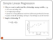
Simple Linear Regression

• Chapter 7

2
Regression Analysis

• A relationship between variables may exist due to
  1 of 4 possible reasons
• Chance
• useless since this relationship can not be
  quantified
• A relationship to a 3rd set of circumstances
• a more direct relationship is desired since it
  provides a better explanation of cost
• A functional relationship
• a precise relationship that seldom exists in cost
  estimating
• A causal type of relationship

3
Definition of Regression

• Regression Analysis is used to describe a
  statistical relationship between variables
• Specifically, it is the process of estimating the
  best fit parameters of a specified function
  that relates a dependent variable to one or more
  independent variables (including implicit
  uncertainty)

y a b x
Regression
Data
y
y
x
x
4
Regression Analysis in Cost Estimating

• If the dependent variable is a cost, the
  regression equation is often referred to as a
  Cost Estimating Relationship or CER
• The independent variable in a CER is often called
  a cost driver
• A CER may have multiple cost drivers

Cost Cost Driver (single)
Aircraft Design of Drawings
Software Lines of Code
Power Cable Linear Feet
CER
3
Examples of cost drivers
CER
Cost Cost Driver (multiple)
Power Cable Linear Feet Power
Example with multiple cost drivers
5
Linear Regression Model

• Cost is the dependent (or unknown) variable
  generally denoted by the symbol Y.
• The systems physical or performance
  characteristics form the models known, or
  independent, variables which are generally
  denoted by the symbol X.
• The linear regression model takes the following
  form
• Yi b0 b1Xi ?i
• where b0 (the Y intercept) and b1 (the slope of
  the regression line) are the unknown regression
  parameters and ?i is a random error term.

• It is assumed that ?I N(0, s2) and iid.

6
Linear Regression Model

• We desire a model of the form
• This model is estimated on the basis of
  historical data as
• b1 and b0 are chosen such that the sum of the
  squared residuals is minimized (Least Squares
  Best Fit).

Y
b
0
Y
b
b
X
0
1
X
1
X
2
X
3
X
7
Least Squares Best Fit (LSBF)

• To find the values of b0 and b1 that minimizes
  one may refer to the Normal
  Equations.
• With two equations and two unknowns, we can solve
  for b0 and b1.

8
An Example

• Suppose were analyzing the production cost of
  radio comm sets.
• The average production cost of all radio comm
  sets in your data set is 250K
• Then you develop an estimating relationship
  between production cost and radio comm set weight
  using LSBF.
• Now you want to estimate the production cost of a
  650 lb. radio comm set.

9
An Example

• What do these numbers mean?
• 250K is the estimate of the average production
  cost of all radio comm sets in the population.
• 311K is the estimate of all radio comm sets in
  the population that have a weight of 650 lbs.

K
311K
311
250
650
lbs
10
Another Example

• Recall the transmogrifier? Now lets look at the
  relationship between transmogrifier weight (lbs)
  and average unit production cost.

11
The Regression Model

• The first time, well crank it out by hand...

12
Standard Error

• Standard Error the standard deviation
  about the regression line. The smaller the
  better.

n-k-1, where k is number of independent variables
25
FY97K
20
15
10
SE
5
SE
0
0
50
100
150
200
Weight (lbs)
13
Standard Error

• For the transmogrifier data, the standard error
  is 5.8K.
• This means that on average when predicting the
  cost of future systems we will be off by 5.8K.

14
Coefficient of Variation

• Coefficient of Variation (CV)
• This says that on average, well be off by 64
  when predicting the cost of future systems. The
  smaller the better.

15
Analysis of Variance

• Analysis of Variance (ANOVA)

16
Analysis of Variance (ANOVA)

• Measures of Variation
• Total Sum of Squares (SST)
• The sum of the squared deviations between the
  data and the average
• Residual or Error Sum of Squares (SSE)
• The sum of the squared deviations between the
  data and the regression line
• The unexplained variation
• Regression Sum of Squares (SSR)
• The sum of the squared deviations between the
  regression line and the average
• The explained variation

7
SST SSE SSR total unexplained
explained
17
Analysis of Variance (ANOVA)

• Mean Measures of Variation
• Mean Squared Error (or Residual) (MSE)
• Mean of Squares of the Regression (MSR)

where n data points k equation parameters
e.g. in our toy problem n 5 and k 2
Y 2.5 0.6 X
The denominator for each of the above is called
the degrees of freedom, or df, associated with
each type of variation
2 parameters
10
5 data points
18
Coefficient of Determination

• Coefficient of Determination (R2) represents the
  percentage of total variation explained by the
  regression model. The larger the better.
• R2 adjusted for degrees of freedom (Adj. R2)
  takes into account the increased uncertainty due
  to a small sample size.

19
The t statistic

• For a regression coefficient, the determination
  of statistical significance is based on a t test
• The test depends on the ratio of the
  coefficients estimated value to its standard
  deviation, called a t statistic
• This statistic tests the marginal contribution of
  the independent variable on the reduction of the
  unexplained variation.
• In other words, it tests the strength of the
  relationship between Y and X (or between Cost and
  Weight) by testing the strength of the
  coefficient b1.
• Another way of looking at this is that the
  t-statistic tells us how many standard deviations
  the coefficient is from zero.
• The t-statistic is used to test the hypothesis
  that X and Y (or Cost and Weight) are NOT related
  at a given level of significance.
• If the test indicates that that X and Y are
  related, then we say we prefer the model with b1
  to the model without b1.

20
The t statistic
0

• Say we wish to test b1 at the a 0.20
  significance level. Refer to Table 6-2 with 8
  degrees of freedom...

• Since our test statistic, 1.97, falls within the
  rejection region, we reject H0 and conclude that
  we prefer the model with b1 to the model without
  b1.

(1 - a) 0.80
a/2 0.10
a/2 0.10
-1.397
b1 0
1.97
1.397
21
The F Statistic

• The F statistic tells us whether the full model
  is preferred to the mean, . That is,
  whether the coefficients of all the independent
  variables are zero
• Say we want to test the strength of the
  relationship between our model and Y at the a
  0.1 significance level...

(1-a) 0.90
From F Table, Pg. 7-50 with 1 numerator and 8
denominator d.o.f.

• Since 3.85 falls within the rejection region, we
  reject H0 and say the full model is better than
  the mean as a predictor of cost.

a 0.10
FC 3.46
0
3.85
22
Theres an Easier Way...

• Linear Regression Results (Microsoft Excel)

• Now the information we need is seen at a glance.

23
Important Results

• From the Excel Regression output we can glean the
  following important results
• R2 or Adj. R2 The bigger the better.
• CV Divide Standard Error by (calculated
  separately). The smaller the better.
• Significance of F If less than a then we prefer
  the model to the mean . Else, vice
  versa.
• P-value of coefficient b1 If less than a then
  we prefer the model with b1, else we prefer it
  without b1.
• These statistics will be used to compare other
  linear models when more than one cost driver may
  exist.

24
Treatment of Outliers

• In general, an outlier is a residual that falls
  greater than 2s from or .
• The standard residual is
• Recall that since 95 of the population falls
  within 2s of the mean, then in any given data
  set, we would expect 5 of the observations to be
  outliers.
• In general, do not throw them out unless they do
  not belong in your population.

25
Outliers with respect to X

• All data should come from the same population.
  You should analyze your observations to ensure
  this is so.
• Observations that are so different that they do
  not qualify as a legitimate member of your
  independent variable population are called
  outliers with respect to the independent
  variable, X.
• To identify outliers with respect to X, simply
  calculate and SX. Those observations that
  fall greater than two standard deviations from
  are likely candidates.
• You expect 5 of your observations to be outlier,
  therefore the fact that some of your observations
  are outliers is not necessarily a problem. You
  are simply identifying observations that warrant
  a closer investigation.

26
Example Analysis of Outliers with Respect to X
27
Outliers with Respect to Y

• There are two types of outliers with respect to
  the dependent variable.
• Those with respect to Y itself.
• Those with respect to the regression model, .
• Outliers with respect to Y itself are treated in
  the same way as those with respect to X.
• Outliers with respect to are of particular
  concern, because those represent observations our
  model does not predict well.
• Outliers with respect to are identified by
  comparing the residuals to the standard error of
  the estimate (SE). This is referred to as the
  standardized residual.
• Outliers are those with residuals greater than 2
  std errors.

28
Remedial Measures

• Remember the fact that you have outliers in your
  data set is not necessarily indicative of a
  problem. The trick is to determine WHY an
  observation is an outlier.
• Possible reasons why an observation is an
  outlier.
• Random Error No problem
• Not a member of the same population If so, you
  want to delete this observation from your data
  set.
• Youve omitted one or more other cost drivers.
• Your model is improperly specified.
• The data point was improperly measured (its just
  plain wrong).
• Unusual event (war, natural disaster).
• A normalization problem.

29
Remedial Measures

• Your first reaction should not be to throw out
  the data point.
• Assuming the observation belongs in the sample,
  some options are
• Dampen or lessen the impact of the observation
  through a transformation of the dependent and or
  independent variables.
• Develop two or more regression equations (with
  and without the outlier)
• Outliers should be treated as useful information.

30
Model Diagnostics

• If the fitted model is appropriate for the data,
  there will be no pattern apparent in the plot of
  the residuals versus Xi, , etc.
• Residuals spread uniformly across the range of
  X-axis values

ei
0
Xi
31
Model Diagnostics

• If the fitted model is not appropriate, a
  relationship between the X-axis values and the ei
  values will be apparent.

32
Example Residual Patterns
Tip A residual plot is the primary way of
indicating whether a non-linear model (and which
one) might be appropriate
Residuals not independent with x A curvilinear
model is probably more appropriate in this case

• Good residual pattern
• Independent with x
• Constant variation

Residuals do not have constant variation Weighted
Least Squares approach should be examined
Residuals not independent with x e.g., in
learning curve analysis, this pattern might
indicate loss of learning or injection of new
work
Usually the residual plot provides enough visual
insight to determine whether or not linear OLS
regression is appropriate. If the picture is
inconclusive, statistical tests exist to help
determine if the OLS assumptions hold1.
33
Non-Linear Models

• Data transformations should be tried when
  residual analysis indicates a non-linear trend
• X??? 1/X X??? 1/Y X??? log X Y???
  ln Y Y??? log Y
• CER is often non-linear when independent variable
  is a performance parameter
• Y aX b
• log Y log a b log X ? Y?? a? bX?
• log-linear transform allows use of linear
  regression
• predicted values for Y are log dollars which
  must be converted
• r2 is potentially misleading when using a log
  model

34
Other Concerns

• When the regression results are illogical (i.e.,
  cost varies inversely with a physical or
  performance parameter), omission of one or more
  important variables may have occurred or the
  variables being used may be interrelated
• Does not necessarily invalidate a linear model
• Additional analysis of the model is necessary to
  determine if additional independent variables
  should be incorporated or if consolidation/elimina
  tion of existing variables is required

35
Assumptions of OLS

• (1) Fixed X
• Can obtain many random samples, each with the
  same X values but different Yi values due to
  different ei values
• (2) Errors have mean of 0
• Eei 0
• (3) Errors have constant variance
  (homoscedasticity)
• Varei s2 for all I
• (4) Errors are uncorrelated
• Covei,ej 0 for all i ? j
• (5) Errors are normally distributed
• ei N(0, s2)