Using LAPS as a CWB Nowcasting Tool

1
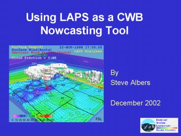
Using LAPS as a CWB Nowcasting Tool

• By
• Steve Albers
• December 2002

2
Local Analysis and Prediction System (LAPS)

• A system designed to
• Exploit all available data sources
• Create analyzed and forecast grids
• Build products for specific forecast applications
• Use advanced display technology
• All within the local weather office

3
LAPS Flow Diagram
4
CWB LAPS Grid

• LAPS Analysis Grid
• Hourly Time Cycle
• Horizontal Resolution 5 km
• Vertical Resolution 50 mb
• Size 199 x 247 x 21

5
Data Acquisition and Quality Control
6
LAPS Data Sources
The blue colored data are currently used in AWIPS
LAPS. The other data are used in the "full-blown"
LAPS and can potentially be added to AWIPS/LAPS
if the data becomes available.
7
LAPS Surface Analysis
8
Multi-layered Quality Control

• Gross Error Checks
• Rough Climatological Estimates
• Station Blacklist
• Dynamical Models
• Use of meso-beta models
• Standard Deviation Check
• Statistical Models (Kalman Filter)
• Buddy Checking

9
Standard Deviation Check

• Compute Standard Deviation of observations-backgro
  und
• Remove outliers
• Now adjustable via namelist

10
Kalman QC Scheme

• FUTURE Upgrade to AWIPS/LAPS QC
• Adaptable to small workstations
• Accommodates models of varying complexity
• Model error is a dynamic quantity within the
  filter, thus the scheme adjusts as model skill
  varies

11
Sfc T
12
CAPE
13
3-D Temperature

• First guess from background model
• Insert RAOB, RASS, and ACARS if available
• 3-Dimensional weighting used
• Insert surface temperature and blend upward
• depending on stability and elevation
• Surface temperature analysis depends on
• METARS, Buoys, and Mesonets (LDAD)

14
Successive correction analysis strategy

• 3-D weighting
• Successive correction with Barnes weighting
• Distance weight e-(d/r)2 applied in 3-dimensions
• Instrument error reflected in observation weight
• Wo e-(d/r)2 / erro2
• Each analysis iteration becomes the background
  for the next iteration
• Decreasing radius of influence (r) with each
  iteration
• Each iteration improves fit and adds finer scale
  structure
• Works well with strongly clustered observations
• Iterations stop when fine scale structure fit
  to obs become commensurate with observation
  spacing and instrument error

15
Successive correction analysis strategy (cont)

• Smooth blending with Background First Guess
• Background subtracted to yield observation
  increments (uo)
• Background (with zero increment) has weight at
  each grid point
• Background weight proportional to inverse square
  of estimated error
• wb 1 / errb2
• For each iteration, analyzed increment (u) is as
  follows
• ui,j,k (uowo) / ( (w o ) wb )

16
X-sectT / Wind
17
LAPS Wind Analysis
18
Products Derived from Wind Analysis
19
Doppler and Other Wind Obs
20
LAPS radar ingest
21
Remapping Strategy

• Polar to Cartesian
• 2D or 3D result (narrowband / wideband)
• Average Z,V of all gates directly illuminating
  each grid box
• QC checks applied
• Typically produces sparse arrays at this stage

22
Remapping Strategy (reflectivity)

• Horizontal Analysis/Filter (Reflectivity)
• Needed for medium/high resolutions (lt5km) at
  distant ranges
• Replace unilluminated points with average of
  immediate grid neighbors (from neighboring
  radials)
• Equivalent to Barnes weighting at medium
  resolutions (5km)
• Extensible to Barnes for high resolutions (1km)
• Vertical Gap Filling (Reflectivity)
• Linear interpolation to fill gaps up to 2km
• Fills in below radar horizon visible echo

23
Mosaicing Strategy (reflectivity)

• Nearest radar with valid data used
• /- 10 minute time window
• Final 3D reflectivity field produced within cloud
  analysis
• Wideband is combined with Level-III
  (NOWRAD/NEXRAD)
• Non-radar data contributes vertical info with
  narrowband
• QC checks including satellite
• Help reduce AP and ground clutter

24
Horizontal Filter/Analysis
Before
After
25
Radar Mosaic
26
LAPS cloud analysis
METAR
METAR
METAR
27
CloudSchematic
28
Cloud Isosurfaces
29
3-D Clouds

• Preliminary analysis from vertical soundings
  derived from METARS, PIREPS, and CO2 Slicing
• IR used to determine cloud top (using temperature
  field)
• Radar data inserted (3-D if available)
• Visible satellite can be used

30
Cloud Analysis Flow Chart
31
Cloud Radar X-sect (Taiwan)
32
Cloud Radar X-sect (wide/narrow band)
33
Derived cloud products flow chart
34
Cloud/Satellite Analysis Data

• 11 micron IR
• 3.9 micron data
• Visible (with terrain albedo)
• CO2-Slicing method (cloud-top pressure)

35
Visible Satellite Impact
36
Cloud Coverage without/with visible data

No vis data
With vis data
37
Storm-Total Precipitation (wideband mosaic)
38
LAPS 3-D Water Vapor (Specific Humidity) Analysis

• Interpolates background field from synoptic-scale
  model forecast
• QCs against LAPS temperature field (eliminates
  possible supersaturation)
• Assimilates RAOB data
• Assimilates boundary layer moisture from LAPS Sfc
  Td analysis

39
LAPS 3-D Water Vapor (Specific Humidity)
Analysis continued

• Scales moisture profile (entire profile excluding
  boundary layer) to agree with derived GOES TPW
  (processed at NESDIS)
• Scales moisture profile at two levels to agree
  with GOES sounder radiances (channels 10, 11,
  12). The levels are 700-500 hPa, and above 500
• Saturates where there are analyzed clouds
• Performs final QC against supersaturation

40
Adjustments to cloud and moisture scheme

• Originally cloud water and ice estimated from
  Smith-Feddes parcel
• Model this tended to produce too much moisture
  and ice
• Adjustments
• Scale vertical motion by diagnosed cloud amount,
  extend below cloud base
• 2. Reduced cloud liquid consistent with 10
  supersaturation of diagnosed water vapor and
  autoconversion rates from Schultz

41
Cloud vertical motions
42
Balance scheme tuned
43
Proposed Tasks for IA15

• Transfer existing LAPS/MM5 Hot-Start system to
  CWB
• LAPS build on LINUX
• Expand satellite and radar data used for cloud
  diagnosis
• Adapt to GOES 9 (visible 3.9 micron)
• Radar data compression needed?
• CWB/NFS as background
• Continued tuning for tropics
• Add thermodynamic constraint to balance package
  to correct for bad background fields
• Add a verification package to the LAPS/MM5 system
  State variables and QPF
• Continue regular upgrades CWB software

44
Sources of LAPS Information

• The Taiwan LAPS homepage
• http//laps.fsl.noaa.gov/taiwan/taiwan_home.html

45
Analysis Information

• LAPS analysis discussions are near the bottom of
• http//laps.fsl.noaa.gov/presentations/presentatio
  ns.html
• Especially noteworthy are the links for
• Satellite Meteorology
• Analyses Temperature, Wind, and Clouds/Precip.
• Modeling and Visualization
• A Collection of Case Studies

46
The End
47
Taiwan Short-Term Forecast System
Taiwan Short Term Forecast System
48
Forecast domains computational requirements
49
CWB Hot-Start MM5 Model Configuration
50
CWB Hot Start Physics
CWB Hot-Start MM5 Model Physics
Initial Field
From LAPS and Diabatic Initialization
Microphysics
Schultz scheme
PBL scheme
MRF PBL
Surface scheme
5-layer Soil Model
Radiation
RRTM scheme
Shallow Convection
YES
Cumulus Parameterization
NO
51
Kalman Flow Chart
52
Cloud Coverage without/with visible data

No vis data
With vis data
53
Case Study Example

• An example of the use of LAPS in convective event
• 14 May 1999
• Location DEN-BOU WFO

54
Case Study Example

• On 14 May, moisture is in place. A line of storms
  develops along the foothills around noon LT (1800
  UTC) and moves east. LAPS used to diagnose
  potential for severe development. A Tornado Watch
  issued by 1900 UTC for portions of eastern CO
  and nearby areas.
• A brief tornado did form in far eastern CO west
  of GLD around 0000 UTC the 15th. Other tornadoes
  occurred later near GLD.

55
NOWRAD and METARS with LAPS surface CAPE 2100 UTC
56
NOWRAD and METARS with LAPS surface CIN 2100 UTC
57
Dewpoint max appears near CAPE max, but between
METARS 2100 UTC
58
Examine soundings near CAPE max at points B, E
and F 2100 UTC
59
Soundings near CAPE max at B, E and F 2100 UTC
60
RUC also has dewpoint max near point E 2100 UTC
61
LAPS RUC sounding comparison at point E (CAPE
Max) 2100 UTC
62
CAPE Maximum persists in same area 2200 UTC
63
CIN minimum in area of CAPE max 2200 UTC
64
Point E, CAPE has increased to 2674 J/kg 2200 UTC
65
Convergence and Equivalent Potential Temperature
are co-located 2100 UTC
66
How does LAPS sfc divergence compare to that of
the RUC? Similar over the plains. 2100 UTC
67
LAPS winds every 10 km, RUC winds every 80
km 2100 UTC
68
Case Study Example (cont.)

• The next images show a series of LAPS soundings
  from near LBF illustrating some dramatic changes
  in the moisture aloft. Why does this occur?

69
LAPS sounding near LBF 1600 UTC
70
LAPS sounding near LBF 1700 UTC
71
LAPS sounding near LBF 1800 UTC
72
LAPS sounding near LBF 2100 UTC
73
Case Study Example (cont.)

• Now we will examine some LAPS cross-sections to
  investigate the changes in moisture, interspersed
  with a sequence of satellite images showing the
  location of the cross-section, C-C (from WSW to
  ENE across DEN)

74
Visible image with LAPS 700 mb temp and wind and
METARS 1500 UTC Note the strong thermal gradient
aloft from NW-S (snowing in southern WY) and the
LL moisture gradient across eastern CO.
75
LAPS Analysis at 1500 UTC, Generated with Volume
Browser
76
Visible image 1600 UTC
77
Visible image 1700 UTC
78
LAPS cross-section 1700 UTC
79
LAPS cross-section 1800 UTC
80
LAPS cross-section 1900 UTC
81
Case Study Example (cont.)

• The cross-sections show some fairly substantial
  changes in mid-level RH. Some of this is related
  to LAPS diagnosis of clouds, but the other
  changes must be caused by the satellite moisture
  analysis between cloudy areas. It is not clear
  how believable some of these are in this case.

82
Case Study Example (cont.)

• Another field that can be monitored with LAPS is
  helicity. A description of LAPS helicity is at
• http//laps.fsl.noaa.gov/frd/laps/LAPB/AWIPS_WFO_p
  age.htm
• A storm motion is derived from the mean wind
  (sfc-300 mb) with an off mean wind motion
  determined by a vector addition of 0.15 x Shear
  vector, set to perpendicular to the mean storm
  motion
• Next well examine some helicity images for this
  case. Combining CAPE and minimum CIN with
  helicity agreed with the path of the supercell
  storm that produced the CO tornado.

83
NOWRAD with METARS and LAPS surface helicity
1900 UTC
84
NOWRAD with METARS and LAPS surface helicity
2000 UTC
85
NOWRAD with METARS and LAPS surface helicity
2100 UTC
86
NOWRAD with METARS and LAPS surface helicity
2200 UTC
87
NOWRAD with METARS and LAPS surface helicity
2300 UTC
88
Case Study Example (cont.)

• Now well show some other LAPS fields that might
  be useful (and some that might not)

89
Divergence compares favorably with the RUC
90
The omega field has considerable detail (which is
highly influenced by topography
91
LAPS Topography
92
Vorticity is a smooth field in LAPS
93
Comparison with the Eta does show some
differences. Are they real?
94
Stay Away from DivQ at 10 km
95
Why Run Models in the Weather Office?

• Diagnose local weather features having mesoscale
  forcing
• sea/mountain breezes
• modulation of synoptic scale features
• Take advantage of high resolution terrain data to
  downscale national model forecasts
• orography is a data source!

96
Why Run Models in the Weather Office? (cont.)

• Take advantage of unique local data
• radar
• surface mesonets
• Have an NWP tool under local control for
  scheduled and special support
• Take advantage of powerful/cheap computers

97
(No Transcript)
98
(No Transcript)
99
SFM forecast showing details of the orographic
precipitation, as well as capturing the Longmont
anticyclone flow on the plains
100
LAPS Summary

• You can see more about our local modeling efforts
  at
• http//laps.fsl.noaa.gov/szoke/lapsreview/start.ht
  ml
• What else in the future? (hopefully a more
  complete input data stream to AWIPS LAPS
  analysis)

101
(No Transcript)
102
(No Transcript)
103
(No Transcript)
104
Reflectivity (800 hPa)
105
Derived products flow chart
106
Cloud/precip cross section
107
Precip type and snow cover
108
Surface Precipitation Accumulation

• Algorithm similar to NEXRAD PPS, but runs
• in Cartesian space
• Rain / Liquid Equivalent
• Z 200 R 1.6
• Snow case use rain/snow ratio dependent on
  column maximum temperature
• Reflectivity limit helps reduce bright band
  effect

109
Storm-Total Precipitation
110
Storm-Total Precipitation (RCWF narrowband)
111
Future Cloud / Radar analysis efforts

• Account for evaporation of radar echoes in dry
  air
• Sub-cloud base for NOWRAD
• Below the radar horizon for full volume
  reflectivity
• Continue adding multiple radars and radar types
• Evaluate Ground Clutter / AP rejection

112
Future Cloud/Radar analysis efforts (cont)

• Consider Terrain Obstructions
• Improve Z-R Relationship
• Convective vs. Stratiform
• Precipitation Analysis
• Improve Sfc Precip coupling to 3D hydrometeors
• Combine radar with other data sources
• Model First Guess
• Rain Gauges
• Satellite Precip Estimates (e.g. GOES/TRMM)

113
Gauge Radar Analysis
114
Gauge Radar Analysis
115
Selected references

• Albers, S., 1995 The LAPS wind analysis. Wea.
  and Forecasting, 10, 342-352.
• Albers, S., J. McGinley, D. Birkenheuer, and J.
  Smart, 1996 The Local Analysis and prediction
  System (LAPS) Analyses of clouds, precipitation
  and temperature. Wea. and Forecasting, 11,
  273-287.
• Birkenheuer, D., B.L. Shaw, S. Albers, E. Szoke,
  2001 Evaluation of local-scale forecasts for
  severe weather of July 20, 2000. Preprints, 14th
  Conf on Numerical Wea. Prediction, Ft.
  Lauderdale, FL, Amer. Meteor. Soc.
• Cram, J.M.,Albers, S., and D. Devenyi, 1996
  Application of a Two-Dimensional Variational
  Scheme to a Meso-beta scale wind analysis.
  Preprints, 15th Conf on Wea. Analysis and
  Forecasting, Norfolk, VA, Amer. Meteor. Soc.
• McGinley, J., S. Albers, D. Birkenheuer, B. Shaw,
  and P. Schultz, 2000 The LAPS water in all
  phases analysis the approach and impacts on
  numerical prediction. Presented at the 5th
  International Symposium on Tropospheric
  Profiling, Adelaide, Australia.
• Schultz, P. and S. Albers, 2001 The use of
  three-dimensional analyses of cloud attributes
  for diabatic initialization of mesoscale models.
  Preprints, 14th Conf on Numerical Wea.
  Prediction, Ft. Lauderdale, FL, Amer. Meteor. Soc.

116
The End
117
Future LAPS analysis work

• Surface obs QC
• Operational use of Kalman filter (with time-space
  conversion)
• Handling of surface stations with known bias
• Improved use of radar data for AWIPS
• Multiple radars
• Wide-band full volume scans
• Use of Doppler velocities
• Obtain observation increments just outside of
  domain
• Implies software restructuring
• Add SST to surface analysis
• Stability indices
• Wet bulb zero, K index, total totals, Showalter,
  LCL (AWIPS)
• LI/CAPE/CIN with different parcels in boundary
  layer
• new (SPC) method for computing storm motions
  feeding to helicity determination
• More-generalized vertical coordinate?

118
Recent analysis improvements

• More generalized 2-D/3-D successive correction
  algorithm
• Utilized on 3-D wind/temperature, most surface
  fields
• Helps with clustered data having varying error
  characteristics
• More efficient for numerous observations
• Tested with SMS
• Gridded analyses feed into variational balancing
  package
• Cloud/Radar analysis
• Mixture of 2D (NEXRAD/NOWRAD low-level) and 3D
  (wide-band volume radar)
• Missing radar data vs no echo handling
• Horizontal radar interpolation between radials
• Improved use of model first guess RH cloud
  liq/ice

119
Cloud type diagnosis
Cloud type is derived as a function of
temperature and stability
120
LAPS data ingest strategy
121
Dummy Image