
Characteristic values - PowerPoint PPT Presentation
Title:
Characteristic values
Description:
Char. eq of a system is det(sI-A)=0 the polynomial det(sI-A) is called char. pol. the roots of char. eq. are char. values they are also the eigen-values of A – PowerPoint PPT presentation
Number of Views:187
Avg rating:3.0/5.0
Title: Characteristic values
1
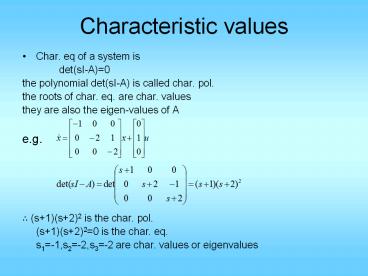
Characteristic values
- Char. eq of a system is
- det(sI-A)0
- the polynomial det(sI-A) is called char. pol.
- the roots of char. eq. are char. values
- they are also the eigen-values of A
- e.g.
- ? (s1)(s2)2 is the char. pol.
- (s1)(s2)20 is the char. eq.
- s1-1,s2-2,s3-2 are char. values or eigenvalues
2
(No Transcript)
3
gtgt MySysss(A,B,C,D) a x1 x2 x3 x1
-1 0 0 x2 0 -2 1 x3 0 0 -2 b
u1 x1 1 x2 0 x3 1 c
x1 x2 x3 y1 1 1 1 d u1
y1 0 Continuous-time model.
gtgt A-1 0 0 0 -2 1 0 0 -2 A -1 0
0 0 -2 1 0 0 -2 gtgt
B101 B 1 0 1 gtgt C1 1
1 C 1 1 1 gtgt D0 D 0
4
gtgt tf(MySys) Transfer function 2 s2 8 s
7 --------------------- s3 5 s2 8 s 4 gtgt
zpk(MySys) Zero/pole/gain 2 (s2.707)
(s1.293) --------------------- (s1)
(s2)2 gtgt roots(2 8 7) ans -2.7071
-1.2929 gtgt roots(1 5 8 4) ans -2.0000
-2.0000 -1.0000
gtgt ssym('s') s s gtgt det(seye(3)-A) ans
(s1)(s2)2 gtgt eig(A) ans -1 -2
-2 gtgt DCinv(seye(3)-A)B ans
1/(s1)1/(s2)21/(s2) gtgt simplify(ans) ans
(2s28s7)/(s1)/(s2)2
5
gtgt inv(seye(3)-A) ans 1/(s1), 0,
0 0,
1/(s2), 1/(s2)2 0,
0, 1/(s2) gtgt ilaplace(ans) ans
exp(-t), 0, 0
0, exp(-2t),
texp(-2t) 0, 0,
exp(-2t) gtgt tsym('t') t t gtgt
expm(At) ans exp(-t), 0,
0 0,
exp(-2t), texp(-2t) 0,
0, exp(-2t)
6
gtgt expm(At)A ans -exp(-t),
0, 0
0,
-2exp(-2t), exp(-2t)-2texp(-2t)
0, 0,
-2exp(-2t) gtgt
Aexpm(At) ans -exp(-t),
0, 0
0,
-2exp(-2t), exp(-2t)-2texp(-2t)
0, 0,
-2exp(-2t) gtgt
Aexpm(At)-expm(At)A ans 0, 0, 0 0,
0, 0 0, 0, 0
7
can
?
set t0
?No
can
?
v
at t0
?
v
8
Solution of state space model
- Recall sX(s)-x(0)AX(s)BU(s)
- (sI-A)X(s)BU(s)x(0)
- X(s)(sI-A)-1BU(s)(sI-A)-1x(0)
- x(t)(L-1(sI-A)-1))Bu(t) L-1(sI-A)-1) x(0)
- x(t) eA(t-t)Bu(t)d teAtx(0)
- y(t) CeA(t-t)Bu(t)d tCeAtx(0)Du(t)
9
S.S to T.F.
- X(s)(sI-A)-1BU(s)
- Y(s)C(sI-A)-1BU(s)DU(s)
- (D C(sI-A)-1B)U(s)
- ? T.F. H(s) D C(sI-A)-1B
- In matlab ss2tf
- eig
- roots
- poly
- use help to find out how to use these
10
- In Matlab
- gtgt A0 1-2 -3
- gtgt B01
- gtgt C1 3
- gtgt D0
- gtgt n,dss2tf(A,B,C,D)
- n
- 0 3.0000 1.0000
- d
- 1 3 2
- gtgttf(n,d)
11
But dont use those for hand calculation
- useX(s)(sI-A)-1BU(s)(sI-A)-1x(0)
- x(t)L-1(sI-A)-1BU(s)L-1 (sI-A)-1
x(0) - Y(s)C(sI-A)-1BU(s)DU(s)C(sI-A)-1x(0)
- y(t) L-1C(sI-A)-1BU(s)DU(s)CL-1
(sI-A)-1 x(0) - e.g.
u unit step
12
Note T.F.D C(sI-A)-1B
13
Eigenvalues, eigenvectors
- Given a nxn square matrix A, p is an eigenvector
of A if Ap?p - i.e. ? s.t. Ap ?p
- ?is an eigenvalue of A
- Example ,
- Let ,
- ?p1 is an e-vector, the e-value1
- Let ,
- ?p2 is also an e-vector, assoc. with the ? -2
14
- In general, if ?, p is an e-pair for A,
- Ap ?p
- ?p-Ap0
- ?Ip-Ap0
- (?I-A)p0
- ? p?0 ? det(?I-A)0
- ? ? is a sol. of char. eq of A
- char. pol. of nxn A has degn
- ? A has n eigen-values.
- e.g. A , det(?I-A)(?-1)(?2)0
- ? ?11, ?2-2
15
- If ?1 ??2 ??3?
- then the corresponding p1, p2, ? will be
linearly independent, i.e., the matrix - Pp1?p2 ? ?pn will be invertible.
- Ap1 ?1p1
- Ap2 ?2p2
- ?
- Ap1?p2 ? ?Ap1?Ap2 ? ?
- ?p1? ?p2 ? ?
- p1 p2 ?
16
- ? APP?
- P-1AP ?diag(?1, ?2, ?)
- ?If A has n lin. ind. Eigenvectors then A can be
diagonalized. - Note Not all square matrices can be diagonalized.
17
(No Transcript)
18
(No Transcript)
19
(No Transcript)
20
(No Transcript)
21
(No Transcript)
22
(No Transcript)
23
(No Transcript)
24
(No Transcript)
25
Example
26
(No Transcript)
27
(No Transcript)
28
- In Matlab
- gtgt A2 0 1
- 0 2 1
- 1 1 4
- gtgt P,Deig(A)
- P
- 0.6280 0.7071 0.3251
- 0.6280 -0.7071 0.3251
- -0.4597 -0.0000 0.8881
- p1 p2 p3
- D
- 1.2679 0 0
- 0 2.0000 0
- 0 0 4.7321
?1
?2
?3
29
- If A does not have n lin. ind. e-vectors
- (some of the eigenvalues are identical),
- then A can not be diagonalized
- E.g. A
- det(?I-A) ?456?31152?210240?32768
- ?1-8
- ?2-16
- ?3-16
- ?4-16
- by solving (?I-A)P0
30
- If we use P,Deig(A)
- get approximate but wrong answer
- Should use gtgtP,Jjordan(A)
- P
- 0.3750 0 1 0.625
- 0 8 4 0
- -0.375 0 0 0.375
- 0 16 9 0
- J
- -8 0 0 0
- 0 -16 1 0
- 0 0 -16 1
- 0 0 0 -16
a 3x3 Jordan block assoc. w/. ?-16
31
More Matlab Examples
- gtgt ssym('s')
- gtgt A0 1-2 -3
- gtgt det(seye(2)-A)
- ans
- s23s2
- gtgt factor(ans)
- ans
- (s2)(s1)
32
- gtgt P,Deig(A)
- P
- 0.7071 -0.4472
- -0.7071 0.8944
- D
- -1 0
- 0 -2
- gtgt P,Djordan(A)
- P
- 2 -1
- -2 2
- D
- -1 0
- 0 -2
33
- A 0 1
- -2 -3
- gtgt exp(A)
- ans
- 1.0000 2.7183
- 0.1353 0.0498
- gtgt expm(A)
- ans
- 0.6004 0.2325
- -0.4651 -0.0972
- gtgt tsym('t')
- gtgt expm(At)
- ans
- -exp(-2t)2exp(-t),
exp(-t)-exp(-2t) - -2exp(-t)2exp(-2t), 2exp(-2t)-exp(-t)
?
34
v
v
35
Similarity transformation
same system as()
36
Example
diagonalized
decoupled
37
Invariance
38
(No Transcript)
39
Controllability
40
Example
41
- In Matlab
- gtgt Sctrb(A,B)
- gtgt rrank(S)
- If S is square (when B is nx1)
- gtgt det(S)
42
Observability
43
Example
44
- In Matlab
- gtgt Vobsv(C,A)
- gtgt rrank(V)
- rank must n
- Or if single output (ie V is square), can use
- gtgt det(V)
- det must be nonzero
Lookfor controllability Lookfor observability
45
(No Transcript)
46
- Recall linear transformation
- Controllabilitybeing able to use u(t) to drive
any state to origin in finite time - Observabilitybeing able to computer any x(0)
from observed y(t) - After transformation, eigenvalues, char. poly,
char. eq, char. values, T.F., poles, zeros
un-changed, but eigenvector changed
47
- Controllability is invariant under transf.
48
(No Transcript)
49
- Observability invariant under transf.
50
(No Transcript)
51
State Feedback
D
1 s
r
u
x
y
B
C
-
A
K
feedback from state x to control u
52
(No Transcript)
53
(No Transcript)
54
- In Matlab
- Given A,B,C,D
- ?Compute QCctrb(A,B)
- ?Check rank(QC)
- If it is n, then
- ?Select any n eigenvalues(must be in complex
conjugate pairs) - ev?1 ?2 ?3 ?n
- ?Compute
- Kplace(A,B,ev)
ABk will have eigenvalues at
55
- Thm Controllability is unchanged after state
feedback. - But observability may change!
Recommended
CrystalGraphics Presentations


