GE5950 Volcano Seismology 13

1
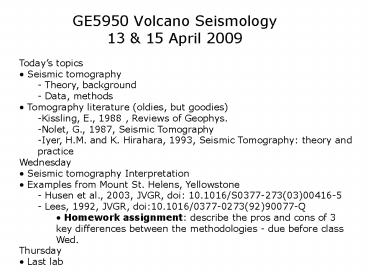
GE5950 Volcano Seismology 13 15 April 2009

• Todays topics
• Seismic tomography
• Theory, background
• Data, methods
• Tomography literature (oldies, but goodies)
• Kissling, E., 1988 , Reviews of Geophys.
• Nolet, G., 1987, Seismic Tomography
• Iyer, H.M. and K. Hirahara, 1993, Seismic
  Tomography theory and practice
• Wednesday
• Seismic tomography Interpretation
• Examples from Mount St. Helens, Yellowstone
• Husen et al., 2003, JVGR, doi
  10.1016/S0377-273(03)00416-5
• Lees, 1992, JVGR, doi10.1016/0377-0273(92)90077-
  Q
• Homework assignment describe the pros and cons
  of 3 key differences between the methodologies -
  due before class Wed.
• Thursday
• Last lab

2
Introduction to Seismic Tomography

• As one of the most widely used seismologists
  tools tomography can be dangerous in the wrong
  hands.
• Why? The striking images one can produce with a
  tomography model are prone to over interpretation
  or misinterpretation.
• Goal for this week is to make you better equipped
  to judge tomography papers for yourselves

3
Introduction to Seismic Tomography

• History
• Name comes from Greek tomos meaning slice plus
  graph
• Adapted from medical CAT scan imaging
• X rays are absorbed
• (attenuated) differently
• by different tissue, bones,
• etc.
• Attenuation is integrated
• along the path of the ray
• Image is constructed
• by discretizing the body into
• small blocks and projecting
• the attenuation back into the
• model
• Lots of data from many
• sources and many receivers

4
Graphical Seismic Tomography

• Imagine a single low velocity anomaly within a
  model

5
Graphical Seismic Tomography

• Because all rays are parallel, there is no
  horizontal resolution

6
Graphical Seismic Tomography

• Adding crossing rays localizes the anomaly

7
Graphical Seismic Tomography

• Adding crossing rays localizes the anomaly

8
Graphical Seismic Tomography

• Adding crossing rays localizes the anomaly

9
Graphical Seismic Tomography

• Need crossing rays

10
Graphical Seismic Tomography

• Real data are more complicated

11
Graphical Seismic Tomography

• Real data are more complicated

12
Introduction to Seismic Tomography

• Adopted for seismic traveltimes in the early
  1970s by, among others Keiiti Aki
• Methodology is well-developed now
• Used at all scales
• Global models
• Large earthquakes
• Regional scale
• Teleseismic earthquakes
• Surface and body waves
• Local
• Shallow high resolution
• Artificial source
• chemical explosion
• Airgun
• Sledge hammer
• Inversion of ambient noise Green functions
• Latest developments use finite frequencies to
  account for the true sensitivity of the wave

13
Why seismic tomography is so difficult

• Raypath is a function of the velocity
• Coverage is not continuous and varies greatly
• Like many problems in geology and geophysics, it
  isnt repeatable
• Source parameters are unknown and have to be
  solved
• These problems are addressed by
• Linearization
• Discretization
• Regularization

14
LET - local earthquake tomography

• Best approach if you dont have Exxon money
• Use local earthquakes as source
• Receivers are typically short-period stations
  deployed for monitoring, earthquake location
• Dozens of studies have been done this way, but it
  is not ideal
• Most of the theory, complications, etc.,
  discussed for LET are the same for all tomography
  studies

15
LET complications

• Earthquake data (sources)
• Earthquakes are not evenly distributed
• Swarms
• Might be only very shallow (deep) in some areas
• Lots of earthquakes in some places, none in
  others
• Fault zones
• Repeated sources recorded at the same receiver
  set do not help

16
Earthquakes are not evenly distributed
17
Earthquakes are not evenly distributed

• Uneven earthquake distribution results in dense
  bands of rays
• These areas are prone to streaking/smearing/trade
  -off

18
LET complications

• Earthquake data (sources)
• Earthquakes are not evenly distributed
• Swarms
• Might be only very shallow (deep) in some areas
• Lots of earthquakes in some places, none in
  others
• Locations are unknown
• Arrival times have uncertainties (pick error)
• Solving for earthquake locations requires that
  you know the velocity structure
• Velocity - hypocenter problem is coupled
• Good starting velocity model is critical

19
LET complications

• Seismic stations (receivers)
• Seismic stations are not evenly distributed
• Near roads or at high points in topography
• At the surface
• Typically are better
• distributed than earthquakes
• Station spacing is
• much larger than
• resolution of interest

20
Earthquake Location

• Remember important criteria for accurate depth
  and epicentral locations?
• Close station
• Small azimithal gap
• Small pick errors
• All we can measure is the arrival time

21
Earthquake Location

• We assume something about the location and
  velocity model to estimate the travel time
• And travel time residual
• For the earthquake location alone, we are solving
  for 4 parameters
• For seismic tomography, we solve for the velocity
  model too

22
Velocity Model

• For each raypath, we have to know the velocity
  all along the raypath from source to receiver
• The traveltime is the integral
• Where s(x,y,z) 1/v(x,y,z) - slowness

23
Velocity Model

• In order to calculate the traveltime, we have to
  discretize the velocity (slowness) model
• The model vector, s, in this example is 1 x 24

24
Velocity Model

• So the traveltime of the ith ray is a summation
  of weighted slowness values

25
The Starting Velocity Model is Critical

• This goes back to the coupled hypocenter-velocity
  problem
• The raypaths depend on the velocity model
• Remember Snellius Law
• Likewise, the earthquake locations depend on the
  staring velocity model
• The velocity model depends on the locations of
  the earthquakes

26
Velocity Model

• Start with simple, smooth 1-D model
• But where does this model come from?
• Usually a 1-D LET inversion
• Many researchers use a minimum 1-D model
• Use a subset (500) of the best-located
  earthquakes
• 10 or more high quality picks
• Small pick uncertainty (lt 5ms for P)
• well-distributed stations (gap lt180, lt 100)
• At least 1 station distance lt 1 times the depth
• Try many different starting models and invert
• The model that produces the lowest total residual
  is the minimum 1-D model

27
The Starting Velocity Model is Critical

• This ray is passing through 4, 7, 8, 11, 14, 15,
  and 18

28
The Starting Velocity Model is Critical

• This ray is passing through 4, 7, 8, 10, 11, 13,
  and 14,
• (Not 15 or 18)

29
Model Discretization

• Once you have a starting 1-D model you have to
  break it up into discrete sections
• Nodes vs. blocks
• Spacing
• Trade-off between spatial resolution of interest
  AND
• Data density
• With smoothing constraint, smaller grid spacing
  might be OK
• For LET,
• horizontal spacing is typically on the order of
  station spacing or smaller
• Vertical spacing is of the same order as
  horizontal but is highly dependent on earthquake
  locations
• Blocks/nodes in areas with poor/no ray coverage
  can be fixed

30
Back to the math

• To calculate the adjustments to the hypocenter
  and velocity model, we need to know how these
  parameters affect the travel time
• The dependency is nonlinear, so we linearize the
  problem by Taylor Series expansion
• Then throw out higher order terms

• hj represents all the hypocenter parameters
• mk represents the velocity model parameters

31
Back to the math

• To calculate the adjustments to the hypocenter
  and velocity model, we need to know how these
  parameters affect the travel time

• ?hj represents changes to the hypocenter
  parameters
• ?mk represents changes to the velocity model
  parameters
• ?F??hj are the linearized partial derivatives
  that describe how the hypocenter parameters
  affect the traveltime
• ?F??mk are the linearized partial derivatives
  that describe how the model parameters affect the
  traveltime

32
Forward and Inverse parts

• The Forward Modeling
• ?F??hj
• ?F??mk
• These have to be solved at each iteration
• Ray tracing can be the computationally most
  expensive part of the inversion
• The Inverse Modeling
• ?hj represents changes to the hypocenter
  parameters
• ?mk represents changes to the velocity model
  parameters

33
The traveltime residual

• Look at this in terms of the traveltime residual
• For the ith travel time residual, ti

34
In matrix form

• ?d G?m
• Where ?d is the vector of traveltime residuals
• G is the matrix of partial derivatives
• Can be separated into hypocenter and model parts,
  but should be solved simultaneously
• ?m is the vector of model parameters

35
Inversion

• ?d G?m
• For ?d lt ?m
• The problem is underdetermined
• Need some smoothing and or damping
• Smoothing keeps the adjacent model parameters
  connected - varying smoothly
• Damping keeps the model parameter close to the
  input model
• For ?d gt ?m
• The problem is overdetermined
• Solve with Least Squares inversion
• ?mGTG-1GT ?d
• Typically use some regularization as well

36
Inversion

• There are lots of resources for details on
  inversion. Two good books
• Menke, 1989
• Zhdanov, 2002
• We wont go into details but, weighted,
  damped or smoothed inversions involve some
  additional terms in the inversion

37
Smoothing and Damping

• Smoothing can be required by the inversion
• How much smoothing is the right amount?

Simons et al., Lithos, 1999
38
Smoothing and Damping

• Smoothing built into the inversion
• Offset-and-average multiple inversions solved
  with different parameterizations
• In the example, we solve for 25 separate models,
  then average

39
Smoothing and Damping

• Smoothing built into the inversion
• Offset-and-average multiple inversions solved
  with different parameterizations
• Graded inversion
• Damping reduces anomalies!
• Iterative inversion should converge on solution
• When to stop iterations?

40
When to stop iterations?

• Usually stop before rms residual error gets below
  the estimated picking error