
Pinhole cameras - PowerPoint PPT Presentation
1 / 65
Title:
Pinhole cameras
Description:
Used in structure from motion. When accuracy really matters, we must model the real camera ... Retina contains cones (mostly used) and rods (for low light) ... – PowerPoint PPT presentation
Number of Views:232
Avg rating:3.0/5.0
Title: Pinhole cameras
1
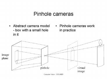
Pinhole cameras
- Abstract camera model - box with a small hole in
it
- Pinhole cameras work in practice
2
Distant objects are smaller
3
Parallel lines meet
Common to draw film plane in front of the focal
point. Moving the film plane merely scales the
image.
4
Vanishing points
- each set of parallel lines (direction) meets at
a different point - The vanishing point for this direction
- Sets of parallel lines on the same plane lead to
collinear vanishing points. - The line is called the horizon for that plane
- Good ways to spot faked images
- scale and perspective dont work
- vanishing points behave badly
- supermarket tabloids are a great source.
5
Slide credit David Jacobs
6
(No Transcript)
7
Properties of Projection
- Points project to points
- Lines project to lines
- Vanishing points for parallel lines
- Parallel lines parallel to image plane donot
converge - Closer objects appear bigger
- Angles are not preserved
- Degenerate cases
- Line through focal point projects to a point.
- Plane through focal point projects to line
8
Pinhole Camera Terminology
Image plane
Optical axis
Principal point/ image center
Focal length
Camera center/ pinhole
Camera point
Image point
9
The equation of projection
10
The equation of projection
- Cartesian coordinates
- We have, by similar triangles, that
(x, y, z) -gt (f x/z, f y/z, -f) - Ignore the third coordinate, and get
11
The camera matrix
- Turn previous expression into HCs
- HCs for 3D point are (X,Y,Z,T)
- HCs for point in image are (U,V,W)
12
Weak perspective
- Issue
- perspective effects, but not over the scale of
individual objects - collect points into a group at about the same
depth, then divide each point by the depth of its
group - Adv easy
- Disadv wrong
13
The Equation of Weak Perspective
- s is constant for all points.
- Parallel lines no longer converge, they remain
parallel.
Slide credit David Jacobs
14
Pros and Cons of These Models
- Weak perspective has simpler math.
- Accurate when object is small and distant.
- Most useful for recognition.
- Pinhole perspective much more accurate for
scenes. - Used in structure from motion.
- When accuracy really matters, we must model the
real camera - Use perspective projection with other calibration
parameters (e.g., radial lens distortion)
Slide credit David Jacobs
15
Orthographic projection
16
The projection matrix for orthographic projection
17
Affine cameras
18
Camera parameters
- Issue
- camera may not be at the origin, looking down the
z-axis - extrinsic parameters
- one unit in camera coordinates may not be the
same as one unit in world coordinates - intrinsic parameters - focal length, principal
point, aspect ratio, angle between axes, etc.
Note the matrix dimensions
19
Camera calibration
- Issues
- what are intrinsic parameters of the camera?
- what is the camera matrix? (intrinsicextrinsic)
- General strategy
- view calibration object
- identify image points
- obtain camera matrix by minimizing error
- obtain intrinsic parameters from camera matrix
- Error minimization
- Linear least squares
- easy problem numerically
- solution can be rather bad
- Minimize image distance
- more difficult numerical problem
- solution usually rather good,
- start with linear least squares
- Numerical scaling is an issue
20
Human Eye
- The eye has an iris like a camera
- Focusing is done by changing shape of lens
- Retina contains cones (mostly used) and rods (for
low light) - The fovea is small region of high resolution
containing mostly cones - Optic nerve 1 million flexible fibres
http//www.cas.vanderbilt.edu/bsci111b/eye/human-e
ye.jpg
Slide credit David Jacobs
21
The Image Formation Pipeline
22
Outline
- Vector, matrix basics
- 2-D point transformations
- Translation, scaling, rotation, shear
- Homogeneous coordinates and transformations
- Homography, affine transformation
23
Notes on Notation
- Vectors, points x, v (assume column vectors)
- Matrices R, T
- Scalars x, a
- Axes, objects X, Y, O
- Coordinate systems W, C
- Number systems R, Z
- Specials
- Transpose operator xT
(as opposed to x0) - Identity matrix Id
- Matrices/vectors of zeroes, ones 0, 1
24
Block Notation for Matrices
- Often convenient to write matrices in terms of
parts - Smaller matrices for blocks
- Row, column vectors for ranges of entries on
rows, columns, respectively - E.g. If A is 3 x 3 and
25
2-D Transformations
- Types
- Scaling
- Rotation
- Shear
- Translation
- Mathematical representation
26
2-D Scaling
27
2-D Scaling
28
2-D Scaling
sx
1
Horizontal shift proportional to horizontal
position
29
2-D Scaling
sy
1
Vertical shift proportional to vertical position
30
2-D Scaling
31
Matrix form of 2-D Scaling
32
2-D Scaling
33
2-D Rotation
34
2-D Rotation
35
2-D Rotation
36
Matrix form of 2-D Rotation
(this is a counterclockwise rotation reverse
signs of sines to get a clockwise one)
37
Matrix form of 2-D Rotation
38
2-D Shear (Horizontal)
39
2-D Shear (Horizontal)
Horizontal displacement proportional to vertical
position
40
2-D Shear (Horizontal)
(Shear factor h is positive for the figure above)
41
2-D Shear (Horizontal)
42
2-D Shear (Vertical)
43
2-D Translation
44
2-D Translation
45
2-D Translation
46
2-D Translation
47
2-D Translation
48
2-D Translation
49
Representing Transformations
- Note that weve defined translation as a vector
addition but rotation, scaling, etc. as matrix
multiplications - Its inconvenient to have two different
operations (addition and multiplication) for
different forms of transformation - It would be desirable for all transformations to
be expressed in a common, linear form (since
matrix multiplications are linear
transformations)
50
Example Trick of additional coordinate makes
this possible
- Old way
- New way
51
Translation Matrix
- We can write the formula using this expanded
transformation matrix as - From now on, assume points are in this expanded
form unless otherwise noted
52
Homogeneous Coordinates
- Expanded form is called homogeneous coordinates
or projective space - Change to projective space by adding a scale
factor (usually but not always 1)
53
Homogeneous Coordinates Projective Space
- Equivalence is defined up to scale (non-zero
for finite points) - Think of projective points in P2 as rays in R3,
where z coordinate is scale factor - All Euclidean points along ray are same in this
sense
54
Leaving Projective Space
- Can go back to non-homogeneous representation by
dividing by scale factor and dropping extra
coordinate - This is the same as saying Where does the ray
intersect the plane defined by z 1? - Analogy to perspective projection, where f1
(image plane) and lambda is z of any point in the
ray. For different lambdas along the line,
projected point is the same, thus Equivalence
class
55
Homogeneous Coordinates Rotations, etc.
- A 2-D rotation, scaling, shear or other
transformation normally expressed by a 2 x 2
matrix R is written in homogeneous coordinates
with the following 3 x 3 matrix - The non-commutativity of matrix multiplication
explains why different transformation orders give
different resultsi.e., RT ? TR
In homogeneous form
In homogeneous form
56
Example Transformations Dont Commute
57
Example Transformations Dont Commute
58
Example Transformations Dont Commute
59
Example Transformations Dont Commute
60
2-D Transformations
- Full-generality 3 x 3 homogeneous transformation
is called a homography
61
2-D Transformations
- Full-generality 3 x 3 homogeneous transformation
is called a homography - Translation components
62
2-D Transformations
- Full-generality 3 x 3 homogeneous
- transformation is called a homography
- Scale/rotation components
63
2-D Transformations
- Full-generality 3 x 3 homogeneous transformation
is called a homography - Shear/rotation components
64
2-D Transformations
- Full-generality 3 x 3 homogeneous transformation
is called a homography - Homogeneous scaling factor
65
2-D Transformations
- Full-generality 3 x 3 homogeneous transformation
is called a homography - When these are zero (as they have been so far), H
is an affine transformation
Recommended
CrystalGraphics Presentations


