Social Networks

1
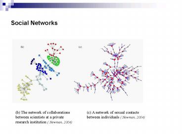
Social Networks
(b) The network of collaborations between
scientists at a private research institution (
Newman, 2004)
(c) A network of sexual contacts between
individuals ( Newman, 2004)
2
Information Networks
Citation Network
World-Wide Web
3
Biological Networks
Metabolic Networks
Protein/Protein Interaction Networks - PPI Yeast
4
Databases of PPI

• MIPS
• Mammalian Protein-Protein Interaction
  Database
• http//mips.gsf.de/proj/ppi/
• DIP
• Database of Interacting Proteins at UCLA.
  No species restriction.
• http//dip.doe-mbi.ucla.edu/
• MINT
• Molecular INTeraction database, Univ. di
  Roma

5
Various types of networks
6
Network Measures Barabási Oltvai, 2004

• Degree Distribution
• Shortest Path and Mean Path Length
• Clustering Coefficient

7
Degree Distribution

• The degree of a vertex in a network is the number
• of edges incident on (i.e., connected to) that
  vertex
• We define p(k) as the probability that a selected
  vertex has exactly k links.
• The histogram of p(k) is the degree distribution
  for the
• network.

8
Cumulative Degree Distribution

• An alternative way of presenting degree data is
  to make a plot of the cumulative distribution
  function
• P(k) ?kk,8 p(k)
• which is the probability that the degree is
  greater than
• or equal to k.
• Such a plot has the advantage that all the
  original data are represented.

9
Degree Distribution in Random Networks

• In a random Erdos and Renyi graph each edge is
  present with equal probability p.
• The degree distribution is, binomial, or Poisson
  in the limit of large graph size.
• The limit of large n is taken holding the mean
  degree
• z p(n - 1) constant

10
Random Network Generation

• To generate a random network, start with N nodes
  and connect each pair of nodes with probability
  p, thus creating a graph with approximately
• 
  pN(N1)/2
• randomly placed links.
• The network has a characteristic degree, close to
  the average degree of the distribution
• There are no highly connected nodes (hubs)

11
Scale-free networks

• The degree distribution approximates a power law
• P(k) k? 2lt?lt3
• The term scale-free" refers to any functional
  form f(x) that remains unchanged to within a
  multiplicative factor under a rescaling of the
  independent variable x, i.e.
• f(ax) bf(x)
• power-law" and scale-free" are synonymous.
• Power-law degree distribution indicates that a
  few hubs hold together numerous small nodes

12
Gaussian versus Power Law

• In a Gaussian distribution most observations are
  around the average the odds of a deviation
  decline faster and faster (exponentially) as we
  move away from the average

13
Examples fromThe Black Swan by Taleb

• Assume average 1.67 meters, and unit of deviation
  10 cm
• Height distribution (a Gaussian quantity)
• 10 cm taller than average 1 in 6.3
• 20 cm taller than average 1 in 44
• 30 cm taller than average 1 in 740
• 40 cm taller than average 1 in 32000
• 50 cm taller than average 1 in 3500000
• ..
• 100 cm taller than average 1 in
  130000000000000000000000
• 110 cm taller than average 1 in
  3600000000000000000000000
• 00000000000000000000000000000000000000000000000000
  00

14
Scalable Wealth Distribution

• People with a net worth
• higher than 1 million 1 in 62.3
• higher than 2 million 1 in 250
• higher than 4 million 1 in 1500
• higher than 8 million 1 in 4000
• higher than 16 million 1 in 16000
• higher than 32 million 1 in 64000
• higher than 16 million 1 in 6400000
• The speed of decrease is constant

15
Wealth Distribution with Large Inequalities

• People with a net worth
• higher than 1 million 1 in 62.3
• higher than 2 million 1 in 125
• higher than 4 million 1 in 250
• higher than 8 million 1 in 500
• higher than 16 million 1 in 1000
• higher than 32 million 1 in 2000
• higher than 320 million 1 in 20000
• higher than 640 million 1 in 40000

16
Wealth Distribution assuming a Gaussian Law

• People with a net worth
• higher than 1 million 1 in 63
• higher than 2 million 1 in 127000
• higher than 4 million 1 in 14000000000
• higher than 8 million 1 in 1600000000000000000000
  0000000000000

17
Power Law A simple property

• P(k) k?
• P(k1)/P(k2) (k1/k2)?
• Example
• Assume ?1.5
• Say that you think that 96 books sell more than
  250000 copies.
• Then you can estimate that x34 books will sell
  more than 500000,
• x/96 (500000/250000)-1.5

18
Assumed exponents for various phenomena (M.E.J.
Newman 2005)

• Frequency of use of words 1.2
• Number of hits on websites 1.4
• Number of books sold in USA 1.5
• Networth of Amerincans 1.1
• Population in US cities 1.3
• People killed in terrorist attacks 2

19
The meaning of the exponent (from The Black
Swan, by Taleb)
20

• For ?gt3 in many respects the scale-free network
  behaves like a random one.

21
Cumulative degree distributions for six
different networks
The horizontal axis is vertex degree k, the
vertical axis is the fraction of vertices that
have degree gt k. (c), (d) and (f), appear to
have power-law degree distributions, (e) has an
exponential degree distribution and (a) appears
to have a truncated power-law degree
distribution
22
Degree Distribution for different types of
networks
23
Clustering or Transitivity

• If vertex A is connected to vertex B and vertex B
  to vertex C, then likely vertex A will also be
  connected to vertex C.
• In social networks, the friend of your friend is
  likely also to be your friend.

24
Clustering Coefficient

• Assume node i has ki adjacent nodes let ni be
  the number of links connecting the neighbours of
  node i to each other. Then
• Ci 2 ni /ki(ki1)
• Alternative definition
• C 3 ? of triangles in the network/?of
  connected triples of vertices

25
Average Cluster Coefficient

• Two definitions
• C ?i Ci
• Average clustering coefficient of all nodes with
  k links
• C(k) ?i Ci (k)

26
Clustering Coefficient

• For many real networks C(k) k 1,
• which is an indication of a networks
  hierarchical character

27
Clustering Coefficients for different types of
networks
28
Mean Path length

• The average over the shortest paths between all
  pairs of nodes
• l 1/(1/2n(n 1)) ?ij dij
• where dij is the length of the shortest path
  (also called geodesic distance) between nodes i
  and j
• A measure of spread of information, networks
  overall navigability, etc.

29
Small-world effect

• A network has the small-world effect if most
  pairs of vertices are connected by a short path
  through the network
• If the number of vertices within a distance r of
  a typical central vertex grows exponentially with
  rand this is true of many networks, including
  the random graph then the value of l will
  increase as log n.
• Networks with power-law degree distributions have
  values of l that increase no faster than log
  n/log log n

30
Selective linking Assortative mixing

• Suppose nodes are classified into different types
  i, i1, ..n.
• Let Eij be the number of edges in the network
  that connect vertices of types i and j, and let E
  be the matrix with elements Eij .
• The normalized matrix e is defined
• e E / E
• where E denotes the sum of all the elements of
  the matrix E. The elements eij measure the
  fraction of edges that fall between vertices of
  types i and j.

31
Assortativity coefficient

• r Tr e e2/ (1 - e2)
• where Tr is the trace of matrix e, i.e. the sum
  of all its diagonal elements
• r is 0 in a randomly mixed network and 1 in a
  perfectly assortative network.

32
Assortativity based on node degree

• Are nodes with high degree preferentially
  connected to each other?
• Social networks are assortative, i.e. well
  connected
• people tend to know each other
• Biological PPI networks and technological WWW
  seem to be disassortativity

33
Assortativity coefficient

• C Pearson correlation coefficient of the degrees
  at either ends of an edge.
• C tends to be positive for assortatively mixed
  networks and negative for disassortative ones.

34
Network clustering
35
Hierarchical Measurements

• Two fundamental operations of mathematical
  morphology
• Dilation
• Erosion

36
Hierarchical Measurements
(a) Dilation the dilation of the initial
subnetwork (dark gray vertices) corresponds to
the dark and light gray vertices (b) Erosion
the erosion of the original subnetwork, given by
the dark gray vertices in (a), results in the
subnetwork represented by the black vertices in
(b).
37
Definitions

• The complement of g is the subgraph implied by
  the set of vertices in G that are not in g.
• The dilation of g is the subgraph d(g)
• implied by the vertices in g plus the vertices
  directly connected to a vertex in g.
• The erosion of g is defined as the complement of
  the dilation of the complement of g

38

• The d-ring of subgraph g, denoted by Rd(g), is
  the subgraph implied by the set of vertices
• N(dd(g)) \ N(dd-1(g))
• The hierarchical degree of a subgraph g at
  distance d can be defined as the number of edges
  connecting rings Rd(g) to Rd1(g).

39
Example