CORE MRP II

1
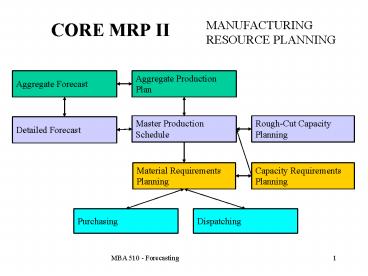
CORE MRP II
MANUFACTURING RESOURCE PLANNING
2
FORECASTING

• Time-series (intrinsic) models
• Time series components
• Base-level forecasting models
• Evaluating forecasting models Mad versus Bias
• Adding trend and seasonality
• Selecting a technique

3
TIME-SERIES (INTRINSIC) FORECASTING MODELS

• Make no assumption about what causes sales
• Identify patterns in past data
• Project those patterns into the future
• Also called autoprojection, intrinsic techniques

4
TIME SERIES COMPONENTS

• Predictable components
• Base level
• Trend
• Seasonality
• Unpredictable components
• Randomness
• All time series techniques work by
• Smoothing randomness out of the past data
•  Projecting the leftover pattern implied by these
  predictable components into the future

5
SHORT-TERM FORECASTING TECHNIQUES

• Assume absence of trend and seasonality
• Separate base-level (average level) from the
  randomness
• Some useful models
• Moving Averages
• Exponential Smoothing

6
BASE-LEVEL FORECASTING MODELS

• Assume absence of trend and seasonality
• Separate base-level from randomness
• Ft -- Forecast for period t
• At -- Actual sales for period t
• Bt -- Base level component for period t
• et -- Random element for period t

7
BASE-LEVEL FORECASTING MODELS

• Example tricycle sales at Bikes-R-Us
• Actual July Sales 105
• True Base level for July 100
• Random spike for July 105-100 5
• Assumption At Bt et 105 100 5
• Practical implications for forecasting
• Step 1 Smooth randomness out of At to estimate
  Bt
• Step 2 Set Ft1 Bt

8
NAÏVE METHOD

• No smoothing of data
• Step 1 Bt At
• Step 2 Ft1 Bt

9
NAÏVE METHOD

• No smoothing of data
• Step 1 Bt At
• Step 2 Ft1 Bt

10
NAÏVE METHOD

• No smoothing of data
• Step 1 Bt At
• Step 2 Ft1 Bt

11
NAÏVE METHOD

• No smoothing of data
• Step 1 Bt At
• Step 2 Ft1 Bt

12
FORECAST EVALUATION

• Need to compare forecast to actual sales
• BIAS
• Too high or to low (on average)?
• Mean Absolute Deviation (MAD)
• Off by how much, per period (on average)?
• Mean Absolute Percentage Error (MAPE)
• A relative measure of MAD

13
FORECAST EVALUATION

• Need to introduce terminology

14
FORECAST EVALUATION
15
FORECAST EVALUATION
16
FORECAST EVALUATION
17
SIMPLE MOVING AVERAGE

• Smoothes out randomness by averaging positive and
  negative random elements over several periods
• n -- number of periods
• Step 1
• Step 2 Ft1 Bt

18
SIMPLE MOVING AVERAGE

• Smoothes out randomness by averaging positive and
  negative random elements over several periods
• n -- number of periods
• Step 1
• Step 2 Ft1 Bt

19
SIMPLE MOVING AVERAGE

• Smoothes out randomness by averaging positive and
  negative random elements over several periods
• n -- number of periods
• Step 1
• Step 2 Ft1 Bt

20
SIMPLE MOVING AVERAGE

• Smoothes out randomness by averaging positive and
  negative random elements over several periods
• n -- number of periods
• Step 1
• Step 2 Ft1 Bt

21
WEIGHTED MOVING AVERAGE

• Same idea as SMA, but less smoothing more
  weight on recent sales data
• n -- number of periods
• ai weight applied to period t-i1
• Step 1
• Step 2 Ft1 Bt

22
WEIGHTED MOVING AVERAGE

• Same idea as SMA, but less smoothing more
  weight on recent sales data
• n -- number of periods
• ai weight applied to period t-i1
• Step 1
• Step 2 Ft1 Bt

23
WEIGHTED MOVING AVERAGE

• Same idea as SMA, but less smoothing more
  weight on recent sales data
• n -- number of periods
• ai weight applied to period t-i1
• Step 1
• Step 2 Ft1 Bt

24
WEIGHTED MOVING AVERAGE

• Same idea as SMA, but less smoothing more
  weight on recent sales data
• n -- number of periods
• ai weight applied to period t-i1
• Step 1
• Step 2 Ft1 Bt

25
EXPONENTIAL SMOOTHING (I)

• Simpler equation, equivalent to WMA
• a exponential smoothing parameter (0lt alt1)
• Step 1
• Step 2 Ft1 Bt

26
EXPONENTIAL SMOOTHING (I)

• Simpler equation, equivalent to WMA
• a exponential smoothing parameter (0lt alt1)
• Step 1
• Step 2 Ft1 Bt

27
EXPONENTIAL SMOOTHING (I)

• Simpler equation, equivalent to WMA
• a exponential smoothing parameter (0lt alt1)
• Step 1
• Step 2 Ft1 Bt

28
EXPONENTIAL SMOOTHING (I)

• Simpler equation, equivalent to WMA
• a exponential smoothing parameter (0lt alt1)
• Step 1
• Step 2 Ft1 Bt

29
EXPONENTIAL SMOOTHING (I)

• Simpler equation, equivalent to WMA
• a exponential smoothing parameter (0lt alt1)
• Step 1
• Step 2 Ft1 Bt

30
EXPONENTIAL SMOOTHING (II)

• A higher smoothing parameter means less smoothing
  and a more reactive forecast

31
E.S. WITH TREND

• Assumes existence of Trend and Base Level
• Tt Trend component in period t
• a Base-level smoothing parameter (0lt alt1)
• b Trend smoothing parameter (0lt blt1)
• Step 1
• Step 2 Ft1 Bt Tt

32
E.S. WITH TREND

• Assumes existence of Trend and Base Level
• Tt Trend component in period t
• a Base-level smoothing parameter (0lt alt1)
• b Trend smoothing parameter (0lt blt1)
• Step 1
• Step 2 Ft1 Bt Tt

33
E.S. WITH TREND

• Assumes existence of Trend and Base Level
• Tt Trend component in period t
• a Base-level smoothing parameter (0lt alt1)
• b Trend smoothing parameter (0lt blt1)
• Step 1
• Step 2 Ft1 Bt Tt

34
E.S. WITH TREND

• Assumes existence of Trend and Base Level
• Tt Trend component in period t
• a Base-level smoothing parameter (0lt alt1)
• b Trend smoothing parameter (0lt blt1)
• Step 1
• Step 2 Ft1 Bt Tt

35
E.S. WITH TREND

• Assumes existence of Trend and Base Level
• Tt Trend component in period t
• a Base-level smoothing parameter (0lt alt1)
• b Trend smoothing parameter (0lt blt1)
• Step 1
• Step 2 Ft1 Bt Tt

36
E.S. WITH TREND

• Assumes existence of Trend and Base Level
• Tt Trend component in period t
• a Base-level smoothing parameter (0lt alt1)
• b Trend smoothing parameter (0lt blt1)
• Step 1
• Step 2 Ft1 Bt Tt

37
E.S. WITH TREND SEASONS

• St Seasonality component in period t
• L Number of seasons in a year
• g Seasonality smoothing parameter (0lt glt1)
• Step 1
• Step 2 Ft1 (Bt Tt )St-L1

38
E.S. WITH TREND SEASONS

• St Seasonality component in period t
• L Number of seasons in a year
• g Seasonality smoothing parameter (0lt glt1)
• Step 1
• Step 2 Ft1 (Bt Tt )St-L1

39
E.S. WITH TREND SEASONS

• St Seasonality component in period t
• L Number of seasons in a year
• g Seasonality smoothing parameter (0lt glt1)
• Step 1
• Step 2 Ft1 (Bt Tt )St-L1

40
E.S. WITH TREND SEASONS

• St Seasonality component in period t
• L Number of seasons in a year
• g Seasonality smoothing parameter (0lt glt1)
• Step 1
• Step 2 Ft1 (Bt Tt )St-L1

41
E.S. WITH TREND SEASONS

• St Seasonality component in period t
• L Number of seasons in a year
• g Seasonality smoothing parameter (0lt glt1)
• Step 1
• Step 2 Ft1 (Bt Tt )St-L1

42
E.S. WITH TREND SEASONS

• St Seasonality component in period t
• L Number of seasons in a year
• g Seasonality smoothing parameter (0lt glt1)
• Step 1
• Step 2 Ft1 (Bt Tt )St-L1

43
E.S. WITH TREND SEASONS

• St Seasonality component in period t
• L Number of seasons in a year
• g Seasonality smoothing parameter (0lt glt1)
• Step 1
• Step 2 Ft1 (Bt Tt )St-L1

44
E.S. WITH TREND SEASONS

• St Seasonality component in period t
• L Number of seasons in a year
• g Seasonality smoothing parameter (0lt glt1)
• Step 1
• Step 2 Ft1 (Bt Tt )St-L1

45
E.S. WITH TREND SEASONS

• St Seasonality component in period t
• L Number of seasons in a year
• g Seasonality smoothing parameter (0lt glt1)
• Step 1
• Step 2 Ft1 (Bt Tt )St-L1

46
E.S. WITH TREND SEASONS

• St Seasonality component in period t
• L Number of seasons in a year
• g Seasonality smoothing parameter (0lt glt1)
• Step 1
• Step 2 Ft1 (Bt Tt )St-L1

47
E.S. WITH TREND SEASONS

• St Seasonality component in period t
• L Number of seasons in a year
• g Seasonality smoothing parameter (0lt glt1)
• Step 1
• Step 2 Ft1 (Bt Tt )St-L1

48
FORECASTING MORE THAN ONE PERIOD AHEAD

• m periods ahead to be forecast
• Base level forecasts Ftm Bt
• Forecasts with trend Ftm Bt mTt
• Forecasts with seasonality Ftm (Bt mTt
  )St-Lm

49
SELECTING A TECHNIQUE

• Ockham's razor -- use the simplest possible model
  or theory (William of Ockham, 1300-1349, England)
• 1) Determine type of technique which is
  appropriate (i.E., Base-level, trend, etc.)
• 2) Select a group of competing techniques which
  satisfy condition (1)
• 3) Select a set of data as a test set
• 4) Simulate forecasts for this set of data using
  all techniques from (2)
• 5) Pick the technique with the best combination
  of MAD/MAPE and Bias