1D%20Pulse%20sequences

1

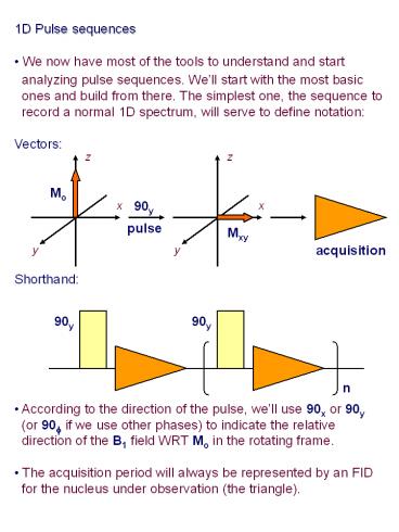
• 1D Pulse sequences
• We now have most of the tools to understand and
  start
• analyzing pulse sequences. Well start with the
  most basic
• ones and build from there. The simplest one,
  the sequence to
• record a normal 1D spectrum, will serve to
  define notation
• Vectors
• Shorthand

z
z
Mo
x
x
90y
pulse
Mxy
y
y
acquisition
90y
90y
n
2

• Inversion recovery
• Measurement of T1 is important, as the
  relaxation rate of
• different nuclei in a molecule can tell us
  about their local
• mobility. We cannot measure it directly on the
  signal or the
• FID because T1 affects magnetization we dont
  detect.
• We use the following pulse sequence
• If we analyze after the p pulse

180y (or x)
90y
tD
z
z
180y (or x)
x
x
tD
y
y
3

• Inversion recovery (continued)

tD 0
z
z
x
x
90y
FT
y
y
tD gt 0
z
z
x
x
90y
FT
y
y
tD gtgt 0
z
z
x
x
90y
FT
y
y
4
Inversion recovery (continued)
at 40oC

• If we plot intensity versus time (td),
• we get the following

I(t) I? ( 1 - 2 e - t / T1 )
Intensity ( )
time
5

• Spin echoes
• In principle, to measure T2 we would only need
  to compute
• the envelope of the FID (or peak width),
  because the signal
• on Mxy, in theory, decays only due to
  transverse relaxation.
• The problem is that the decay we see on Mxy is
  not only due
• to relaxation, but also due to inhomogeneities
  on Bo (the
• dephasing of the signal). The decay constant we
  see on the
• FID is called T2. To measure T2 properly we
  need to use
• spin echoes.
• The pulse sequence looks like this

180y (or x)
90y
tD
tD
6

• Spin echoes (continued)
• We do the analysis after the 90y pulse

z
y
y
tD
x
?
x
x
y
dephasing
y
y
tD
x
x
180y (or x)
refocusing
z
y
?
x
y
7

• Spin echoes (continued)
• If we acquire an FID right after the echo, the
  intensity of the
• signal after FT will affected only by T2
  relaxation and not by
• dephasing due to an inhomogeneous Bo. We repeat
  this for
• different tDs and plot the intensity against 2
  tD. In this case
• its a simple exponential decay, and fitting
  gives us T2.

at 90oC
Intensity ( )
I(t) Io e - t / T2
time
8

• Applications of spin echo sequences
• So far we havent discussed how chemical shift
  and coupling
• constants behave during spin echos. Here well
  start seeing
• how useful they are...
• A pretty anoying thing we have to do in NMR
  spectroscopy is
• phase the spectrum. Why do we have to do this?
  We have to
• think on the effects of chemical shift on
  different components
• of Mxy during a short time or delay.
• This short delay, called the pre-acquisition
  delay (DE), is
• needed or otherwise the remants of the high
  power pulse
• will give us artifacts in the spectrum or burn
  the receivers.

y
y
...
?
x
x
9

• Spectrum phasing
• The phase of the lines appears due to the
  contribution of
• absorptive or real (cosines) and dispersive or
  imaginary
• (sines) components of the FID. Depending on the
  relative
• frequencies of the lines, well have more or
  less sine/cosine
• components
• S(w)x S cosines(w) - real
  spectrum
• S(w)y S sines(w) - imaginary
  spectrum
• What we want is the purely absorptive spectrum,
  so we
• combine different amounts of the real (cosine)
  and the
• imaginary (sine) signals obtained by the
  detector. The
• combination depends on the frequency of the
  spectrum

10

• Spin-echoes on chemical shift
• Now we go back to our spin-echoes. The effects
  on elements
• of Mxy with an offset from the B1 frequency are
  analogous to
• those seen for dephased Mxy after the p / 2
  pulse
• After a time tD, the magnetization precesses in
  the ltxygt
• plane weff tD (f) radians, were weff w -
  wo. After the p pulse
• and a second period tD, the magnetization
  precesses the
• same amount back to the x axis.

z
y
y
tD
x
?
x
x
f
y
weff
y
y
180
tD
x
?
x
f
weff
11

• Spin-echoes and heteronuclear coupling
• We now start looking at more interesting cases.
  Consider a
• 13C nuclei coupled to a 1H
• If we took the 13C spectrum we would see the
  lines split due
• to coupling to 1H. The 1JCH couplings are from
  50 to 250 Hz,
• and make the spectrum really complicated and
  overlapped.
• We usually decouple the 1H, which means that we
  saturate
• 1H transitions. The 13C multiplets are now
  single lines

J (Hz)
bCbH
13C
aCbH
1H
1H
bCaH
I
13C
aCaH
bCbH
13C
aCbH
1H
1H
bCaH
13C
I
aCaH
12

• Spin-echoes and heteronuclear coupling ()
• We modify a little our pulse sequence to include
  decoupling
• Now we analyze what this combination of pulses
  will do to
• the 13C magnetization in different cases. We
  first consider a
• CH (a methine carbon). After the p / 2 pulse,
  we will have
• the 13C Mxy evolving under the action of J
  coupling. Each

180y (or x)
90y
tD
tD
13C
1H
1H
z
y
y
- J / 2
(a)
tD
?
x
x
f
x
y
(b)
J / 2
13

• Spin-echoes and heteronuclear coupling ()
• We now apply the p pulse, which inverts the
  magnetization,
• and start decoupling 1H. This removes the
  labels of the two
• vectors, and effectively stops them. They
  collapse into one,
• with opposing components canceling out
• In this case the second tD under decoupling of
  1H is there to
• refocus chemical shift and get nice phasing
• Now, if we take different spectra for several tD
  values and plot

y
y
y
?
?
x
x
x
tD 1 / 2J
tD 1 / J
tD
14

• Spin-echoes and heteronuclear coupling ()
• The signal intensity varies with the cosine of
  tD, is zero for tD
• values equal to multiples of 1 / 2J and
  maximum/minimum
• for multiples of 1 / J.
• If we are looking at a CH2 (methylene), the
  analysis is
• similar, and we obtain the following plot of
  amplitudes versus
• delay times

tD 1 / 2J
tD
tD 1 / J
tD 1 / 2J
tD 1 / J
tD
15

• Spin-echoes and heteronuclear coupling ()
• Now, if we make the assumption that all 1JCH
  couplings
• are more or less the same (true to a certain
  degree), and
• use the pulse sequence on the following
  molecule with a tD
• of 1 / J, we get (dont take the d values for
  granted)

5
3
7
2
4
6
6
1
1,4
0 ppm
150
100
50
5
2,3
7
16

• Spin-echoes and homonulcear coupling
• Here well see why spin echoes wont work if we
  want to get
• our perfectly phased spectrum. The problem is
  that so far we
• have only used single lines (no homonuclear J
  coupling) or
• systems that have heteronuclear coupling.
• Lets consider a 1H that is coupled to another
  1H, and that we
• are exactly on resonance. After the p / 2 pulse
  of the spin-
• echo sequence and the td delay we have
  evolution under the
• effects of J coupling. Each vector will be
  labeled by the state
• of the 1H it is coupled to. We have

z
J / 2
y
y
(a)
tD
?
x
x
x
y
(b)
J / 2
17

• Spin-echoes and homonulcear coupling ()
• The p pulse flips the vectors and inverts the
  labels
• Now, instead of refocusing, things start moving
  backwards,
• and we will have even more separation of the
  lines of the
• multiplet during the second evolution period.
  If we then take
• the FID, the signal will be completely
  dispersive (although
• this depends on the length of the tD periods)

J / 2
J / 2
y
y
(a)
(b)
180y (or x)
x
x
(b)
(a)
J / 2
J / 2
y
tD
FID, FT
x
18

• Spin-echoes and homonulcear coupling ()
• We see why this is not all that useful. For
  different td values
• we get the following lineshapes for a doublet
  coupled with
• a triplet (both have the same J value)

19

• Binomial pulses
• Binomial pulses are examples of pulse trains
  which we can
• explain with vectors. Among other things, we
  can use them
• to eliminate solvent peaks (see T1).
• The simplest binomial pulse is the 11, two p /
  2 pulses with
• opposite signs, separated by a certain interval
  td, and exactly
• on resonance with the peak we want to
  eliminate
• The first p / 2 puts everything on ltxygt. After
  td, signals/spins
• precess to one side or the other of x. All
  except the signal we

z
z
y
Mo
90y
tD
x
x
x
y
y
20

• Binomial pulses (continued)
• The next p / 2 return everything on x to the z
  axis. This
• includes all the signal corresponding to the
  peak to eliminate,
• as well as the x components of the remaining
  signals
• The resulting FID only has signals corresponding
  to peaks
• that arent in resonance with the carrier. They
  will all be in
• phase with the receiver, but signals on each
  side of the
• carrier will have opposite signs

y
y
90-y
?
x
x
x
y
y
FID (y) FT
x
21

• Binomial pulses ()
• As mentioned before, they are used to eliminate
  solvent
• peaks, particularly water in cases that other
  secuences could
• perturb protons that exchange with water (NHs,
  OHs, etc.).
• 50 mM sucrose in H2O/D2O (9 to 1).
• 1H spectrum

22

• Binomial pulses ()
• To avoid the sign change we can use other
  binomial pulse
• trains, such as the 1331
• You also get artifacts. None of these pulse
  trains, nor
• experiments that take advantage on T1
  differences, give
• results as good as those that are obtained with
  secuences
• using gradients, such as WEFT or WATERGATE.
• For the same sample this is what we get with
  WEFT