NP-Complete Problems (Fun part)

1
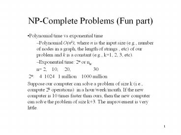
NP-Complete Problems (Fun part)

• Polynomial time vs exponential time
• Polynomial O(nk), where n is the input size
  (e.g., number of nodes in a graph, the length of
  strings , etc) of our problem and k is a constant
  (e.g., k1, 2, 3, etc).
• Exponential time 2n or nn.
• n 2, 10, 20, 30
• 2n 4 1024 1 million 1000 million
• Suppose our computer can solve a problem of size
  k (i.e., compute 2k operations) in a
  hour/week/month. If the new computer is 10 times
  faster than ours, then the new computer can solve
  the problem of size k3. The improvement is very
  little.

2
Story

• All algorithms we have studied so far are
  polynomial time algorithms.
• Facts people have not yet found any polynomial
  time algorithms for some famous problems, (e.g.,
  Hamilton Circuit, longest simple path, Steiner
  trees).
• Question Do there exist polynomial time
  algorithms for those famous problems.
• Answer No body knows.

3
Story

• Research topic Prove that polynomial time
  algorithms do not exist for those famous
  problems, e.g., Hamilton circuit problem.
• You can get Turing award if you can give the
  proof.
• In order to answer the above question, people
  define two classes of problems, P class and NP
  class.
• To answer if P?NP, a rich area, NP-completeness
  theory is developed.

4
Class P and Class NP

• Class P contains those problems that are solvable
  in polynomial time.
• They are problems that can be solved in O(nk)
  time, where n is the input size and k is a
  constant.
• Class NP consists of those problem that are
  verifiable in polynomial time.
• What we mean here is that if we were somehow
  given a solution, then we can verify that the
  solution is correct in time polynomial in the
  size of the input to the problem.
• Example Hamilton Circuit given (v1, v2, , vn),
  we can test if (vi, v i1) is an edge in G and
  (vn, v1) is an edge in G.

5
Class P and Class NP

• Based on definitions, P?NP.
• If we can design an polynomial time algorithm for
  problem A, then problem A is in P.
• However, if we have not been able to design a
  polynomial time algorithm for problem A, then
  there are two possibilities
• polynomial time algorithm does not exists for
  problem A and
• we are too dump.

6
NP-Complete

• A problem is NP-complete if it is in NP and is
  as hard as any problem in NP.
• If an NP-complete problem can be solved
  polynomial time, then any problem in class NP
  can be solved in polynomial time.
• NPC problems are the hardest in class NP.
• The first NPC problem is Satisfiability probelm
• Proved by Cook in 1971 and obtains the Turing
  Award for this work
• Definition of Satisfiability problem Input A
  boolean formula f(x1, x2, xn), where xi is a
  boolean variable (either 0 or 1). Question

7
Boolean formula

• A boolean formula f(x1, x2, xn), where xi are
  boolean variables (either 0 or 1), contains
  boolean variables and boolean operations AND, OR
  and NOT .
• Clause variables and their negations are
  connected with OR operation, e.g., (x1 OR NOTx2
  OR x5)
• Conjunctive normal form of boolean formula
• contains m clauses connected with AND
  operation.
• Example
• (x1 OR NOT x2) AND (x1 OR NOT x3 OR x6) AND
  (x2 OR x6) AND (NOT x3 OR x5).
• Here we have four clauses.

8
Satisfiability problem

• Input conjunctive normal form with n variables,
  x1, x2, , xn.
• Problem find an assignment of x1, x2, , xn
  (setting each xi to be 0 or 1) such that the
  formula is true (satisfied).
• Example conjunctive normal form is
• (x1 OR NOTx2) AND (NOT x1 OR x3).
• The formula is true for assignment
• x11, x20, x31.

9
Satisfiability problem

• Theorem Satisfiability problem is NP-complete.
• It is the first NP-complete problem.
• S. A. Cook in 1971
• Won Turing prize for this work.
• Significance
• If Satisfiability problem can be solved in
  polynomial time, then ALL problems in class NP
  can be solved in polynomial time.
• If you want to solve P?NP, then you should work
  on NPC problems such as satisfiability problem.
• We can use the first NPC problem, Satisfiability
  problem, to show that other problems are also
  NP-complete.

10
How to show that a problem is NPC?

• To show that problem A is NP-complete, we can
• First find a problem B that has been proved to be
  NP-complete.
• Show that if Problem A can be solved in
  polynomial time, then problem B can also be
  solved in polynomial time.
• Remarks Since A NPC problem is the hardest in
  class NP, problem A is also the hardest
• Example We know that Hamilton circuit problem
  is NP-complete. (See a research paper.) We want
  to show that TSP problem is NP-complete.
• .

11
Hamilton circuit and Traveling Salesman problem

• Hamilton circuit a circle uses every vertex of
  the graph exactly once except for the last
  vertex, which duplicates the first vertex.
• It was shown to be NP-complete.
• Traveling Salesman problem (TSP) Input Vv1,
  v2, ..., vn be a set of nodes (cities) in a
  graph and d(vi, vj) the distance between vi
  and vj,, find a shortest circuit that visits
  each city exactly once.
• (weighted version of Hamilton circuit)
• Theorem 1 TSP is NP-complete.

12
Proof of Theorem 1.

• Proof Given any graph G(V, E) (input of
  Hamilton circuit problem), we can construct an
  input for the TSP problem as follows
• For each edge (vi, vj) in E, we assign a
  distance d(vi, vj) 1.
• The new problem becomes that is there a shortest
  circuit that visits each city (node) exactly
  once?
• The length of the shortest circuit is V since
  we need V edges to form the circuit and the
  length of each edge is 1.
• Note The reduction (transformation) is from
  Hamilton circuit (known to be NPC) to the new
  problem TSP (that we want to prove it to be NPC).
  

13
Some basic NP-complete problems

• 3-Satisfiability Each clause contains at most
  three variavles or their negations.
• Vertex Cover Given a graph G(V, E), find a
  subset V of V such that for each edge (u, v) in
  E, at least one of u and v is in V and the size
  of V is minimized.
• Hamilton Circuit (definition was given before)
• History Satisfiability?3-Satisfiability?vertex
  cover?Hamilton circuit.
• Those proofs are very hard.
• Karp proves the first few NPC problems and
  obtains Turing award.

14
Approximation Algorithms

• Concepts
• Steiner Minimum Tree
• TSP
• Knapsack
• Vertex Cover

15
Concepts of Approximation Algorithms

• Optimization Problem
• An optimization problem ? consists of the
  following three parts
• A set D? of instances
• for each instance I?D?, a set S?(I) of candidate
  solutions for I and
• a function C that assigns to each solution
  s(I)?S?(I) a positive number C(s(I)), called the
  solution value (or the cost of the solution).

16

• Maximization
• An optimal solution is a candidate solution
  s(I)?S?(I) such that C(s(I))C(s'(I)) for any
  s'(I)?S?(I).

• Minimization
• An optimal solution is a candidate solution
  s(I)?S?(I) such that C(s(I))C(s'(I)) for any
  s'(I)?S?(I).

17
Approximation Algorithm

• An algorithm A is an approximation algorithm for
  ? if, given any instance I?D?, it finds a
  candidate solution s(I)?S?(I).
• How good an approximation algorithm is?
• We use performance ratio to measure the
  "goodness" of an approximation algorithm.

18
Performance ratio

• For minimization problem, the performance ratio
  of algorithm A is defined as a number r such that
  for any instance I of the problem,
• where OPT(I) is the value of the optimal solution
  for instance I and A(I) is the value of the
  solution returned by algorithm A on instance I.

19
Performance ratio

• For maximization problem, the performance ratio
  of algorithm A is defined as a number r such that
  for any instance I of the problem,
• OPT(I)
• A(I)
• is at most r, where OPT(I) is the value of
  the optimal solution for instance I and A(I) is
  the value of the solution returned by algorithm A
  on instance I.

20
Simplified Knapsack Problem

• Given a finite set U of items, a size s(u)?Z, a
  capacity Bmaxs(u)u?U, find a subset U'?U such
  that and such that the above summation is as
  large as possible. (It is NP-hard.)

21
Ratio-2 Algorithm

• Sort u's based on s(u)'s in increasing order.
• Select the smallest remaining u until no more u
  can be added.
• Compare the total value of selected items with
  the item with the largest size, and select the
  larger one.
• Theorem The algorithm has performance ratio 2.

22
Proof

• Case 1 the total of selected items 0.5B (got
  it!)
• Case 2 the total of selected items lt 0.5B.
• In this case, the size of the largest remaining
  item gt0.5B. (Otherwise, we can add it in.)
• Selecting the largest item gives ratio-2.

23
The 0-1 Knapsack problem

• The 0-1 knapsack problem
• N items, where the i-th item is worth vi dollars
  and weight wi pounds.
• vi and wi are integers.
• A thief can carry at most W (integer) pounds.
• How to take as valuable a load as possible.
• An item cannot be divided into pieces.
• The fractional knapsack problem
• The same setting, but the thief can take
  fractions of items.

24
Ratio-2 Algorithm

• Delete the items I with wigtW.
• Sort items in decreasing order based on vi/wi.
• Select the first k items item 1, item 2, , item
  k such that
• w1w2, wk ?W and w1w2, wk w
  k1gtW.
• 4. Compare vk1 with v1v2vk and select the
  larger one.
• Theorem The algorithm has performance ratio 2.

25
Proof of ratio 2

• C(opt) the cost of optimum solution
• C(fopt) the optimal cost of the fractional
  version.
• C(opt)?C(fopt).
• v1v2vk v k1gt C(fopt).
• So, either v1v2vk gt0.5 C(fopt)?c(opt)
• or v k1 gt0.5 C(fopt)?c(opt).
• Since the algorithm choose the larger one from
  v1v2vk and v k1
• We know that the cost of the solution obtained by
  the algorithm is at least 0.5 C(fopt)?c(opt).

26
Steiner Minimum Tree

• Steiner minimum tree in the plane
• Input a set of points R (regular points) in the
  plane.
• Output a tree with smallest weight which
  contains all the nodes in R.
• Weight weight on an edge connecting two points
  (x1,y1) and (x2,y2) in the plane is defined as
  the Euclidean distance

27

• Example Dark points are regular points.

28
Triangle inequality

• Key for our approximation algorithm.
• For any three points in the plane, we have
• dist(a, c ) dist(a, b) dist(b, c).
• Examples

c
5
4
a
b
3
29
Approximation algorithm(Steiner minimum tree in
the plane)

• Compute a minimum spanning tree for R as the
  approximation solution for the Steiner minimum
  tree problem.
• How good the algorithm is? (in terms of the
  quality of the solutions)
• Theorem The performance ratio of the
  approximation algorithm is 2.

30
Proof

• We want to show that for any instance (input) I,
  A(I)/OPT(I) r (r1), where A(I) is the cost of
  the solution obtained from our spanning tree
  algorithm, and OPT(I) is the cost of an optimal
  solution.

31

• Assume that T is the optimal solution for
  instance I. Consider a traversal of T.

• Each edge in T is visited at most twice. Thus,
  the total weight of the traversal is at most
  twice of the weight of T, i.e.,
• w(traversal)2w(T)2OPT(I). .........(1)

32

• Based on the traversal, we can get a spanning
  tree ST as follows (Directly connect two nodes
  in R based on the visited order of the traversal.)

From triangle inequality, w(ST)w(traversal)
2OPT(I). ..........(2)
33

• Inequality(2) says that the cost of the spanning
  tree ST is less than or equal to the cost of an
  optimal solution.
• So, if we can compute ST, then we can get a
  solution with cost2OPT(I).(Great! But finding
  ST may also be very hard, since ST is obtained
  from the optimal solution T, which we do not
  know.)
• We can find a minimum spanning tree MT for R in
  polynomial time.
• By definition of MST, w(MT) w(ST) 2OPT(I).
• Therefore, the performance ratio is 2.

34
Story

• The method was known long time ago. The
  performance ratio was conjectured to be
• Du and Hwang proved that the conjecture is true.

35
Graph Steiner minimum tree

• Input a graph G(V,E), a weight w(e) for each
  e?E, and a subset R?V.
• Output a tree with minimum weight which contains
  all the nodes in R.
• The nodes in R are called regular points. Note
  that, the Steiner minimum tree could contain some
  nodes in V-R and the nodes in V-R are called
  Steiner points.

36

• Example Let G be shown in Figure a. Ra,b,c.
  The Steiner minimum tree T(a,d),(b,d),(c,d)
  which is shown in Figure b.
• Theorem Graph Steiner minimum tree problem is
  NP-complete.

37
Approximation algorithm(Graph Steiner minimum
tree)

1. For each pair of nodes u and v in R, compute the
   shortest path from u to v and assign the cost of
   the shortest path from u to v as the length of
   edge (u, v). (a complete graph is given)
2. Compute a minimum spanning tree for the modified
   complete graph.
3. Include the nodes in the shortest paths used.

38

• Theorem The performance ratio of this algorithm
  is 2.
• Proof
• We only have to prove that Triangle Inequality
  holds. If
• dist(a,c)gtdist(a,b)dist(b,c) ......(3)
• then we modify the path from a to c like
• a?b?c
• Thus, (3) is impossible.

39

• Example II-1

g
a
e
c
d
f
b
The given graph
40

• Example II-2

e-c-g /7
g /3
e /4
a
c
d
f/ 2
e /3
b
f-c-g/5
Modified complete graph
41

• Example II-3

g/3
a
c
d
f /2
e /3
b
The minimum spanning tree
42

• Example II-4

g
2
1
2
a
e
c
d
1
1
f
b
1
The approximate Steiner tree
43
Approximation Algorithm for TSP with triangle
inequality

• Assumption the triangle inequality holds. That
  is, d (a, c) d (a, b) d (b, c).
• This condition is met, for example, whenever the
  cities are points in the plane and the distance
  between two points is the Euclidean distance.

44

• The above assumption is very strong, since we
  assume that the underline graph is a complete
  graph. Example II does not satisfy the
  assumption. If we want to use the cost of the
  shortest path between two vertices as the cost,
  we have to repeat some nodes.
• Theorem TSP with triangle inequality is also
  NP-hard.

45
Ratio 2 Algorithm

• Algorithm A
• Compute a minimum spanning tree algorithm (Figure
  a)
• Visit all the cities by traversing twice around
  the tree. This visits some cities more than once.
  (Figure b)
• Shortcut the tour by going directly to the next
  unvisited city. (Figure c)

46

• Example

47
Proof of Ratio 2

1. The cost of a minimum spanning tree cost(t), is
   not greater than opt(TSP), the cost of an optimal
   TSP. (Why? n-1 edges in a spanning tree. n edges
   in TSP. Delete one edge in TSP, we get a spanning
   tree. Minimum spanning tree has the smallest
   cost.)
2. The cost of the TSP produced by our algorithm is
   less than 2cost(T) and thus is less than
   2opt(TSP).

48

• Another description of Algorithm A
• Compute a minimum spanning tree algorithm.
• Convert the spanning tree into an Eulerian graph
  by doubling each edge of the tree.
• Find an Eulerian tour of the resulting graph.
• Convert the Eulerian tour into traveling salesman
  tour by using shortcuts.
• Review An Eulerian graph is a graph in which
  every vertex has even degree.

49
Ratio 1.5 Algorithm

• Modify Step 2 as follows
• Let V'a1,a2,...,a2k be the set of vertices
  with odd degree. (There are even number of odd
  degree vertices)
• Find a minimum weight matching for V' in the
  induced graph.
• The cost of the minimum match is at most 0.5
  times of that of TSP. (Why?)

50

• Adding the match to the spanning tree, we get an
  Eulerian graph.
• The cost of the Euler circuit is less than
  1.5opt(TSP).
• The shortcut (i.e., the TSP) produced in step 4
  has a cost not greater than that of the Euler
  circuit produced in step 3.
• So, the TSP produced by our algorithm has a
  cost1.5opt(TSP).

51
Non-approximatility for TSP without triangle
inequality

• Theorem For any xgt0, TSP problem without
  triangle inequality cannot be approximated within
  ratio x.

52

• Example
• Solid edges are the original edges in the graph
  G.
• Dashed edges are added edges.
• OPTn-1 if a Hamilton circuit exists. Otherwise,
  OPTgt2xn.
• Since ratiox, if our solutionlt2xn, Hamilton
  circuit exists.

53
Proof

• The basic idea
• Show that if there is an approximation algorithm
  A with ratio x for TSP problem without triangle
  inequality, then we can use the approximation
  algorithm A for TSP to solve the Hamilton
  Circuit problem, which is NP-hard.
• Since NP-hard problems do not have any polynomial
  time algorithms, the ratio x approximation
  algorithm can not exist.

54

1. Given an instance of Hamilton Circuit problem
   G(V,E), where there are n nodes in V, we assign
   weight 1 to each edge in E. (That is, the
   distance between any pair of vertices in G is 1
   if there is an edge connecting them.)
2. Add edges of cost 2xn to G such that the
   resulting graph G'(V,E?E') is a complete graph.

55

• 3. Now, we use the approximation algorithm A for
  TSP to find a TSP.
• 4. Now, we want to show that if the cost of the
  solution obtained from A is not greater than
  1xn, then there is a Hamilton circuit in G,
  otherwise, there is no Hamilton Circuit in G.

56

• If A gives a solution of cost not greater than
  1xn, then no added edge (weight 2xn) is used.
• Thus, G has a Hamilton circuit.
• If the cost of the solution given by A is greater
  than 1xn, then at least one added edge is used.
• If there is a circuit in G, the cost of an
  optimal solution is n. The approximation
  algorithm A should give a solution with cost
  xn.
• There is no Hamilton circuit in G.

57
Vertex Cover Problem

• Given a graph G(V, E), find V'?V such that for
  each edge (u, v)?E at least one of u and v
  belongs to V.
• V' is called vertex cover.
• The problem is NP-hard.

58
Ratio-2 Approximation Algorithm

• Based on maximal matching
• A match M is a set of edges in E such that no two
  edges in M incident upon the same node in V.
• Maximal matching A matching E' is maximal if
  every remaining edge in E-E' has an endpoint in
  common with some member of E'.

59

• Computation of maximal match
• Add edge to E' until no longer possible.
• Facts
• The 2E' nodes in E' form a cover.
• The optimal vertex cover contains at least E'
  nodes.
• From 1 and 2, the ratio is 2.

60
Assignment

• Question 3. A graph is given as follows.

61

• Use the ratio 1.5 algorithm to compute a TSP.
  (When do shortcutting, if there is no edge, add
  an edge with cost that is equal to the cost of
  the corresponding path.)