
Verification of FSM Equivalence - PowerPoint PPT Presentation
1 / 19
Title:
Verification of FSM Equivalence
Description:
... any state in Ri-1 since we have already found all successor ... (Ri-1 is the set of currently reached states and g is the vector of next state functions) ... – PowerPoint PPT presentation
Number of Views:26
Avg rating:3.0/5.0
Title: Verification of FSM Equivalence
1
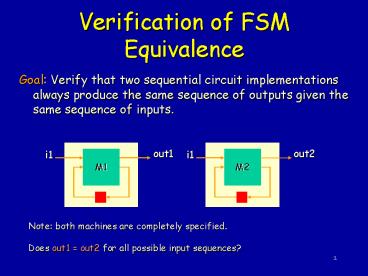
Verification of FSM Equivalence
- Goal Verify that two sequential circuit
implementations always produce the same sequence
of outputs given the same sequence of inputs.
out2
out1
i1
i1
M2
M1
Note both machines are completely
specified. Does out1 out2 for all possible
input sequences?
2
FSM Equivalence of the Product Machine
- Form the product machine
- M(S,I,T,O,Init) x (x1,x2) present
state y (y1,y2) next state - i i1 i2 input Init(x)
(Init1(x1) x Init2(x2)) initial states T(x,i,y)
T1(x1,i,y1) ? T2(x2,i,y2) transition
relation f(x,i) (f1(x1,i) ? f2(x2,i))
single outputwhere ? denotes XNOR operation.
3
Implicit State Enumeration
- The FSMs are equivalent iff for all inputs,
their outputs are identical on all reachable
state pairs. - Let R be the set of all reachable state pairs.
- Equivalence is verified by the following
predicate ?(x,i) (x? R) ? f(x,i) - Easy computation with BDDs. Simply compute
f(x,i)and check if this is identically 1.
4
Implicit State Enumeration
- The following fixed point algorithm computes the
set of reachable state pairs R(x) of an
FSM.R0(x) Init(x)Rk1(x) Rk(x) y ? x
?x, i (Rk(x) ? T(x,i,y))where y ? x represents
substitution of x for y. - The iteration terminates when Rk1(x) Rk(x) and
the least fixed point is reached.
5
Implicit FSM Traversal
- Implicit enumeration of reached state set
- manipulates set of states directly in a BFS
manner - exponential speed-up over explicit enumeration
methods (sometimes) - exploits the fact that the number of states does
not usually reflect system complexity - implicit state enumeration may take a long time
for sequentially deep circuits e.g. those with
counters
one set of states at a time
one step
6
Finding Reachable States in an FSM
R0 is the set of intial states
R0
7
Finding Reachable States in an FSM
R1 is the set of states reachable from the
initial states in less than or equal to one steps.
R1
8
Finding Reachable States in an FSM
R2 is the set of states reachable from the
initial states in less than or equal to two steps.
R2
9
Finding Reachable States in an FSM
The fixed-point iteration terminates after
finding R4 R5. The resultant set is the set
of reachable states.
R2
R4R5
10
Partial Product Method
- Do not need to compute the transition relation
T(x,i,y) explicitly as a single monolithic BDD. - Can keep T(x,i,y) in product form (called
partitioned translation relation)
11
Partial Product Method Using Constrain
- Can form the constrain with respect to Rk(x) of
each (yj ? fj) before forming the final AND. This
usually reduces the size of the final AND. - The final AND operation can be decomposed into a
balanced binary tree of Boolean ANDs. - intermediate variables can be quantified out as
soon as no other product depends on those
variables.
12
Using Constrain
- Can pre-cluster groups of Tj(xj,ij,yj) (defined
as (yj ? fj(xj,ij))) together Cj
?ikj(Tj1,...,Tjk)where the ikj that we can
quantify out here are the ones that do not appear
in any other Ti. Thus - Using constrain is a bad idea since
(Cj(xj,ij,yj))Rk(x) may result in a BDD with more
variables. (It is better to use RESTRICT).
13
Better Idea Use Restrict
- Linearly order (heuristically) the Cj and
multiply from the right by Rk(x) one at a time,
quantifying variables xq, iq as soon as possible
(when they appear in no other terms). - Ri1 Ri(x) y ? x ?(xp,ip)Cl1(...(?(xq,iq
) ClqPi(x))...) - where Pi(x) RESTRICT(Ri, ).
- Note here we do not care about any state in Ri-1
since we have already found all successor states
of these. - Computation done as a binary tree where
quantification of x and i is done as soon as
possible
Quantify all remaining variables that appear in
no other remaining node.
ClqPi(x)
14
End of lecture 25
15
Restrict Operator
- Restrict
- if f is independent of xi then RESTRICT(f,c) is
also. - it does not have the other nice properties of
constrain. - Experiments show that restrict produces smaller
BDDs.
function RESTRICT(f,c) assert(c ? 0) if (c 1
or is_constant(f)) return f else if (cxi 0),
return RESTRICT(fxi,cxi) else if (cxi 0),
return RESTRICT(fxi,cxi) else if (fxi fxi),
return RESTRICT(fxi, cxi cxi) else return xi
RESTRICT(fxi,cxi) xi RESTRICT(fxi,cxi)
16
Recursive Image Method
- (Ri-1 is the set of currently reached states and
g is the vector of next state functions) - The method uses CONSTRAIN Let
- g Bn ? Bm, g g1, g2, ..., gm, and
- c characteristic function of Ri-1 .
- First step use the CONSTRAIN operator to form f
gc (g1)c, (g2)c, ..., (gm)c. - Second step the range of f is determined. Let
R(f) denote the range of the function f. - Ri R(f)(y) y1R(f2,...,fmf1)
y1R(f2,...,fmf1)
17
Explicit FSM Traversal
- Explicit enumeration
- process one state at a time
- for each state, next states are enumerated one by
one - complexity depends on the number of states and
the number of input values. - methods that enumerate the state space explicitly
cannot handle FSMs with a large number of states
first
1
one state at a time
second
2
third
3
fourth
4
18
State enumeration
- State traversal techniques are essential to
- synthesis of sequential circuits
- verification of sequential circuits
- Applications
- sequential testing Cho, Hachtel and Somenzi ITC
91 - extraction of sequential dont cares
- implementation verification
- checking sequential equivalence Coudert and
Madre ICCAD 90 Touati, Lin, Brayton and
Sangiovanni ICCAD 90 - design verification
- checking language containment of ?-regular
languages Touati, Kurshan and Brayton 1991
HSIS system 94 - CTL model checking Burch, Clarke, McMillan and
Dill DAC 90 SMV (CMU 91), VIS (Berkeley 96),
MOCHA (Berkeley 98) systems
19
End of this section
20
FSM Equivalence on the Product Machine
21
Transition and Output Relations
- Let x be the present state, i the inputs, y the
next state, and o the outputs. - Transition function vector f(x,i) f1(x,i),
..., fm(x,i) - Output relationO(x,i,o) 1 ? output is o at
state x and input i - Transition relationT(x,i,y) 1 ? y next
state from state x on input i. - Note transition relation can represent
non-deterministic FSM but transition functions
cannot.
22
Transition and Output Relations
m
(
)
(
)
(
)
Õ
º
i
x
f
y
y
i
x
T
,
,
,
k
k
k
1
y1
f1
?
x
y2
f2
T(x,i,y)
?
y3
f3
?
ym
i
Transition Relation
fm
?
23
Range, Domain, Image and Inverse Image
- R(f) range of f and D(f) domain f(x) is a
unique point y ? R, but f-1(y) is in general a
set - The image of a function f(x) with respect to a
domain constraint C(x) is denoted Img (f, C)
y ?x ? C y f(x).In terms of relation
T(x,i,y) and BDD operators Img (T, C)(y)
?x(C(x) ? T(x,i,y)). - The inverse image of a function f(x) with respect
to a domain constraint C(y) is denoted Pre (f,
C) x ?y ? C y f(x).In terms of
relation T(x,i,y) and BDD operators Pre (T,
C)(x) ? y(C(y) ? T(x,i,y)). - Img (T,C) and Pre (T,C) are sets usually
represented by BDDs.
24
Generalized Cofactor
- Recall
- If c is a cube, the Shannon cofactor is the cover
of the generalized cofactor cof(f,c), which is
independent of variables of the cube c. - There are many other functions which cover
cof(f,c). - Want heuristic to select a representative
function of cof(f,c) that has a small BDD
representation. - The constrain operator Coudert ICCAD 90 is a
representation of generalized cofactor which, in
most cases, has a small BDD representation. - When c is a cube, constrain operator gives the
same result as the usual Shannon cofactor.
25
Constrain Operator
- function constrain(f,c) assert(c ? 0) if (c 1
or is_constant(f)) return f else if (cxi 0),
return constrain(fxi,cxi) else if (cxi 0),
return constrain(fxi,cxi) else return xi
constrain(fxi,cxi) xi constrain(fxi,cxi)
26
Properties of Constrain Operator
- Following properties of the constrain operator
make it very useful in implicit image
computations. We denote constrain(f,c) by fc. - (g ? f)c g ? fcIn particular, (f g)c fc
gc and (f)c (fc). - ?x f(x,y) ? c(x) ?x fc(x,y)
- c is contained in f iff fc is a tautology.
- If c is the characteristic function of a set A ?
Bn, then fc(Bn) f(A). i.e. R(fc) Img (f,A) - Given F (f,d,r), fd usually has a smaller BDD
representation than f.
27
Constrain Operator Another Perspective
- Let c Bn ? B be a non-null Boolean function,
and x1 lt x2 lt ... lt xn an ordering of its input
variables. The mapping ?c is defined as follows - ?c is a projection that maps a minterm x ? Bn to
a minterm y in the ON-set of c, which has the
closest distance to x, according to the distance
metric d. - The particular metric used guarantees the
uniqueness of y in the definition above. - Since ?c maps all points in Bn into the ON-set of
c, then fc(x) f(?c(x)). If f (f1,...,fm),
then fc ((f1)c,...,(fm)c).
28
Fixed Point Iteration via Predicate Transformers
- Let (p,q) be two predicates on a finite set S.
Let F be a predicate transformer, i.e. F(p) r
where r is a new predicate on S. Suppose F is
monotone p ? q ? F(p) ? F(q)We associate a
sequence pi as follows p0 0 pi1
F(pi) p? pi if pi1 pi p? is called the
least fixed point of the predicate transformer F. - Note that pi ? pi1, since 0 ? F(p0) ? F(0) ?
F(F(0)). - Since S is finite (pi)i?0 converges after a
finite number of iterations.
29
Fixed Point Iteration via Predicate Transformers
- If p0 S, the corresponding iteration gives the
greatest fixed point of F. - All sets can be represented by BDDs, and the
predicate transformer F(pi) can be computed using
BDD operations.
Recommended
CrystalGraphics Presentations


