Chapter 5 and 6 Probability Distributions and Normal Probability Distributions

1
Chapter 5 and 6 Probability Distributions and
Normal Probability Distributions
2
Chapter Goals
Combine the ideas of frequency distributions and
probability to form probability distributions

• Learn about the normal, bell-shaped, or Gaussian
  distribution

• How probabilities are found

• How probabilities are represented

• How normal distributions are used in the real
  world

3
5.2 Random Variables

• Random Variable A variable that assumes a unique
  numerical value for each of the outcomes in the
  sample space of a probability experiment

4
Examples of Random Variable

• 1. Let the number of computers sold per day by a
  local merchant be a random variable. Integer
  values ranging from zero to about 50 are possible
  values.

2. Let the number of pages in a mystery novel at
a bookstore be a random variable. The smallest
number of pages is 125 while the largest number
of pages is 547.
3. Let the time it takes an employee to get to
work be a random variable. Possible values are
15 minutes to over 2 hours.
4. Let the volume of water used by a household
during a month be a random variable. Amounts
range up to several thousand gallons.
5. Let the number of defective components in a
shipment of 1000 be a random variable. Values
range from 0 to 1000.
5
Discrete Continuous Random Variables

• Discrete Random Variable A quantitative random
  variable that can assume a countable number of
  values

• Intuitively, a discrete random variable can
  assume values corresponding to isolated points
  along a line interval. That is, there is a gap
  between any two values.

Note Usually associated with counting
Continuous Random Variable A quantitative random
variable that can assume an uncountable number of
values

• Intuitively, a continuous random variable can
  assume any value along a line interval, including
  every possible value between any two values

Note Usually associated with a measurement
6
Example

• Example Determine whether the following random
  variables are discrete or continuous

1. The barometric pressure at 1200 PM 2. The
length of time it takes to complete a statistics
exam 3. The number of items in the shopping cart
of the person in front of you at the checkout
line 4. The weight of a home grown
zucchini 5. The number of tickets issued by the
PA State Police during a 24 hour period 6. The
number of cans of soda pop dispensed by a machine
placed in the Mathematics building on
campus 7. The number of cavities the dentist
discovers during your next visit
7
Probability Distribution Function

• Probability Distribution A distribution of the
  probabilities associated with each of the values
  of a random variable. The probability
  distribution is a theoretical distribution it is
  used to represent populations.

• Notes
• The probability distribution tells you everything
  you need to know about the random variable.
• The probability distribution may be presented in
  the form of a table, chart, function, etc.

Probability Function A rule that assigns
probabilities to the values of the random variable
8
6.2 Normal Probability Distributions

• The normal probability distribution is the most
  important distribution in all of statistics

• Many continuous random variables have normal or
  approximately normal distributions

• Need to learn how to describe a normal
  probability distribution

9
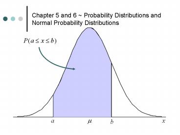
Normal Probability Distribution

• 1. A continuous random variable

3. Recall the probability that x lies in some
interval is the area under the curve
10
The Normal Probability Distribution
11
Notation

• If x is a normal random variable with mean m and
  standard deviation s, this is often denoted x
  N(m, s2)

• Example Suppose x is a normal random variable
  with m 35 and s 6. A convenient notation to
  identify this random variable is x N(35, 62).

12
Probabilities for a Normal Distribution
13
Percentage, Proportion Probability

• Percentage (30) is usually used when talking
  about a proportion (3/10) of a population

• Probability is usually used when talking about
  the chance that the next individual item will
  possess a certain property

• Area is the graphic representation of all three
  when we draw a picture to illustrate the situation

14
6.3 Standard Normal Distribution

• Properties
• The total area under the normal curve is equal to
  1
• The distribution is mounded and symmetric it
  extends indefinitely in both directions,
  approaching but never touching the horizontal
  axis
• The distribution has a mean of 0 and a standard
  deviation of 1
• The mean divides the area in half, 0.50 on each
  side
• Nearly all the area is between z -3.00 and z
  3.00

• Notes
• Table 3, Appendix B lists the probabilities
  associated with the intervals from the mean (0)
  to a specific value of z
• Probabilities of other intervals are found using
  the table entries, addition, subtraction, and
  the properties above

15
Table 3, Appendix B Entries

• The table contains the area under the standard
  normal curve between 0 and a specific value of z

16
Example

• Example Find the area under the standard normal
  curve between z 0 and z 1.45

17
Example

• Example Find the area under the normal curve to
  the right of z 1.45 P(z gt 1.45)

18
Example

• Example Find the area to the left of z 1.45
  P(z lt 1.45)

19
Notes

• The symmetry of the normal distribution is a key
  factor in determining probabilities associated
  with values below (to the left of) the mean. For
  example the area between the mean and z -1.37
  is exactly the same as the area between the mean
  and z 1.37.

• When finding normal distribution probabilities, a
  sketch is always helpful

20
Example

• Example Find the area between the mean (z 0)
  and z -1.26

21
Example

• Example Find the area to the left of -0.98 P(z
  lt -0.98)

22
Example

• Example Find the area between z -2.30 and z
  1.80

23
Example

• Example Find the area between z -1.40 and z
  -0.50

24
Normal Distribution Note

• The normal distribution table may also be used to
  determine a z-score if we are given the area
  (working backwards)

• Example What is the z-score associated with the
  85th percentile?

25
Solution

• In Table 3 Appendix B, find the area entry that
  is closest to 0.3500

. . .
. . .

• The area entry closest to 0.3500 is 0.3508
• The z-score that corresponds to this area is 1.04
• The 85th percentile in a standard normal
  distribution is 1.04

26
Example

• Example What z-scores bound the middle 90 of a
  standard normal distribution?

27
Solution

• The 90 is split into two equal parts by the
  mean. Find the area in Table 3 closest to 0.4500

• 0.4500 is exactly half way between 0.4495 and
  0.4505
• Therefore, z 1.645
• z -1.645 and z 1.645 bound the middle 90 of
  a normal distribution

28
6.4 Applications of Normal Distributions

• Apply the techniques learned for the z
  distribution to all normal distributions

• Start with a probability question in terms
  ofx-values

• Convert, or transform, the question into an
  equivalent probability statement
  involvingz-values

29
Standardization

• Suppose x is a normal random variable with mean m
  and standard deviation s

30
Example

• Example A bottling machine is adjusted to fill
  bottles with a mean of 32.0 oz of soda and
  standard deviation of 0.02. Assume the amount
  of fill is normally distributed and a bottle is
  selected at random

1) Find the probability the bottle contains
between 32.00 oz and 32.025 oz 2) Find the
probability the bottle contains more than 31.97 oz
31
Solution Continued
32
Example, Part 2
2)
33
Notes

• The normal table may be used to answer many kinds
  of questions involving a normal distribution

• Often we need to find a cutoff point a value of
  x such that there is a certain probability in a
  specified interval defined by x

• Example The waiting time x at a certain bank is
  approximately normally distributed with a mean
  of 3.7 minutes and a standard deviation of 1.4
  minutes. The bank would like to claim that 95
  of all customers are waited on by a teller
  within c minutes. Find the value of c that
  makes this statement true.

34
Solution
35
Example

• Example A radar unit is used to measure the
  speed of automobiles on an expressway during
  rush-hour traffic. The speeds of individual
  automobiles are normally distributed with a mean
  of 62 mph. Find the standard deviation of all
  speeds if 3 of the automobiles travel faster
  than 72 mph.

36
Solution
-
m
x


z


s
.

1
88
10
s