
TEMPERATURE LAPSE RATE THE STANDARD ATMOSPHERE - PowerPoint PPT Presentation
1 / 31
Title:
TEMPERATURE LAPSE RATE THE STANDARD ATMOSPHERE
Description:
For 45, the (sin )-1 correction becomes increasingly inaccurate. ... virtual source below the ground at (x0, y0, -z0) that is the mirror image of the ... – PowerPoint PPT presentation
Number of Views:57
Avg rating:3.0/5.0
Title: TEMPERATURE LAPSE RATE THE STANDARD ATMOSPHERE
1
(No Transcript)
2
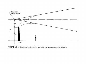
PLUME RISE
- H h ??h
- h physical stack height, ?
- ?h plume rise due to thermal buoyancy and
momentum - Correlations of various complexity exist between
plume rise, stack temperature, stack velocity,
atmospheric conditions etc. (e.g. Hollands,
equation 6.35 de Nevers)
3
PLUME RISE - HOLLANDS EQUATION
4
PLUME RISE - BUOYANCY AND MOMENTUM FLUXES
5
Table 4-6 Wark, Warner Davis
- Equations for calculating final plume rise
6
STACK TIP DOWNWASH
- For Vs lt 1.5 us
- (Vs stack gas velocity, us wind velocity at stack
height) - Note that maximum downwash correction is 3 stack
diameters
7
BUILDING DOWNWASH AND WAKE EFFECTS
- Figs. 3-19 and 3-20 demonstrate these. Special
treatments are included in models. - BUILDING DOWNWASH - Simple rule of thumb
- downwash unlikely to be a problem if
- hs ? hb 1.5 Lb
- hs stack height
- hb building height
- Lb the lesser of either building height or
maximum projected building width. - Good Engineering Practice (GEP) rule for stack
design.
8
(No Transcript)
9
(No Transcript)
10
LINE SOURCES - Infinite line source
- Can be handled in principle as one dimensional
dispersion from a point source. - For wind perpendicular to line source
- q emission per unit time per unit distance
11
Oblique wind and finite line source
- For wind at an angle of ? with the line source,
the strength is effectively increased by a
factor of - (sin ? )-1
- For a finite line source we must consider the end
effects, the resulting concentration will be less
than that for an infinite line source under the
same conditions. - Examples 4-9 and 4-10 (Wark, Warner Davis)
demonstrate the application of the infinite line
source case to CO concentrations near a highway.
12
(No Transcript)
13
(No Transcript)
14
(No Transcript)
15
COMPLICATIONS
- For ? lt 45, the (sin ? )-1 correction becomes
increasingly inaccurate. - The dispersion due to vehicle induced turbulence
and thermal buoyancy due to heat release from
the vehicles are important factors - The P-G-T dispersion coefficients were originally
observed in flat grass terrain, most highways of
interest have some roughness effects associated
with them (bridge, below grade. above grade etc.)
16
CALINE
- series of models developed to provide better
estimations of motor vehicle pollutant
concentrations near highways and arteries. - Main features
- - Finite line segment approach
- - Mixing zone concept to incorporate traffic
induced dispersion - - New dispersion data near highways,
adjustments for averaging time and surface
roughness included for P-G-T coefficients
17
3 DIMENSIONAL DISPERSION MODEL
- Similar to heat conduction equation in 3-d
- Solution for instantaneous release of X g of
pollutant at t 0 and x y z 0
18
PUFF RELEASE
- Solution for instantaneous release of X g of
pollutant at t 0 and (x0, y0, z0) - Using ? instead of K, we get
19
PUFF RELEASE
- To consider ground reflection we add a virtual
source below the ground at (x0, y0, -z0) that is
the mirror image of the real source above the
ground.
Virtual source to account for reflection
20
- At z 0 (cwith reflection ) 2(cwithout
reflection ) - Not as simple at other z.
21
PUFF RELEASE
- Say we release a puff at ground level (z00)
- The center of the plume (y00) is travelling in
the x direction with windspeed u, i.e. x0 ut - Ground-level concentration (z0) along the center
line of the plume, y0 , will be given by
22
PUFF RELEASE
- Ground-level concentration will be at a maximum
for xx0 i.e
23
(No Transcript)
24
(No Transcript)
25
(No Transcript)
26
Decay of pollutants in the atmosphere
- The mass balances we have used so far assume
conservative pollutants no generation or
consumption terms. - For a reactant being consumed by a first order
reaction in a batch reactor
27
Decay of pollutants in the atmosphere
- The time spent in the atmosphere after release
x/u - Thus, first order decay in the atmosphere can be
modelled simply by
28
ATMOSPHERIC TURBULENCE AND SAMPLING TIME
- The time scale for atmospheric turbulence can be
quite long, of the order of many minutes. - Field observations of dispersion coefficients are
specific to the sampling (averaging) time used
(typically 10 minutes) - Estimates of corrections for other sampling
periods can be made
29
(No Transcript)
30
(No Transcript)
31
- From Air Dispersion Modelling Guideline for
Ontario, Guidance for Demonstrating Compliance
with The Air Dispersion Modelling Requirements
set out in Ontario Regulation 419/05, Air
pollution Local Air Quality, made under the
Environmental Protection Act, July 2005. - Available at http//www.ene.gov.on.ca/envision/ai
r/regulations/localquality.htm