
Scaling Relationships in Biology including Community Ecology - PowerPoint PPT Presentation
1 / 41
Title: Scaling Relationships in Biology including Community Ecology
1
Scaling Relationships in Biology(including
Community Ecology)
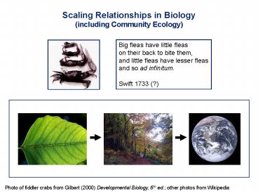
Big fleas have little fleas on their back to bite
them, and little fleas have lesser fleas and so
ad infinitum. Swift 1733 (?)
Photo of fiddler crabs from Gilbert (2000)
Developmental Biology, 6th ed. other photos from
Wikipedia
2
Scaling Relationships
Organisms range over 21 orders of magnitude in
body size!
Statistic from West et al. (1997) Fig. from
Bonner (1988)
3
Scaling Relationships
Biologically relevant processes operate over an
enormous range of spatial temporal scales
Figure from Levin (1992)
4
Scaling Relationships
For example gas exchange through individual
stomata global warming represent phenomena that
occur at vastly different scales of space time
Processes are naturally linked across scales, so
how can we extrapolate from one scale to another
(e.g., leaf ? forest ? globe)?
What are the mechanistic links among patterns and
processes across scales?
Photos from Wikipedia
5
Scaling Relationships
A good starting point is to identify scaling
relationships
Scaling often assesses how attributes change with
changes in a fundamental dimension (e.g.,
length, mass, time)
The attributes of the organism, community or
ecosystem are generally the dependent variables
(Y), whereas the fundamental dimension is the
independent variable (X)
6
Scaling Relationships
Many scaling relationships can be expressed as
power laws Y c Xs X is the independent
variable measured in units of a fundamental
dimension c is a constant of proportionality and
s is the exponent (or power of the function)
The relationship is a straight line on a log-log
plot Log10(Y) Log10(c) s ? Log10(X) and
by rearranging, this is the form of the familiar
equation for a straight line y mx b
7
Scaling Relationships
Consider the scaling of squares cubes as
functions of the length of a side (the
fundamental dimension)
Area Length2 Area ? Length2
Surface area 6 Length2 Surface area ? Length2
Volume Length3 Volume ? Length3
8
Scaling Relationships
Y X2 (accelerating function)
Area
Length
9
Scaling Relationships
Y X2 (accelerating function)
Area
Length
10
Scaling Relationships
Y X2 (accelerating function)
Area
Length
11
Scaling Relationships
Y X2 (accelerating function)
Y 2X
Log10(Area)
Area
Length
Log10(Length)
Etc
12
Scaling Relationships
Y 2X 0.778
Y 6 X2 (accelerating function)
Log10(Surface Area)
Surface area
Length
Log10(Length)
Etc
13
Scaling Relationships
Y X3 (accelerating function)
Y 3X
Volume
Log10(Volume)
Length
Log10(Length)
Etc
14
Scaling Relationships
Consider the ways in which surface area
volume of a sphere scale with its radius
Surface area 4 ? r2 Surface area ? r2
Volume 4/3 ? r3 Volume ? r3
15
Scaling Relationships
Surface-to-volume ratio Surface area
? r2 ? Surface area1/2 ? r Volume ?
r3 ? Volume1/3 ? r
Surface area1/2 ? Volume1/3 ? Surface area
? Volume2/3
16
Scaling Relationships
Slope 1
Y4.83 X0.667
Y0.667 X 0.68
Surface area
Log10(Surface area)
(decelerating function)
Log10(Volume)
Volume
Volume increases proportionately faster than
surface area
Etc
17
Scaling Relationships
Slope 1
Y4.83 X0.667
Y0.667 X 0.68
Surface area
Log10(Surface area)
(decelerating function)
Volume
Log10(Volume)
This simple fact has myriad important
implications for biology
Etc
18
Scaling Relationships
Slope 1
Y4.83 X0.667
Y0.667 X 0.68
Surface area
Log10(Surface area)
(decelerating function)
Volume
Log10(Volume)
For example, endoparasite S should increase more
rapidly than ectoparasite S as host body size
increases
Etc
19
Scaling Relationships
Y 3 X-1
Surface area / Volume
Radius
As you could infer from the earlier figures, the
surface area to volume ratio changes with the
radius of the sphere
Etc
20
Scaling Relationships
Y 3 X-1
Y -1 X 0.48
Log10(Surface area / Volume)
Surface area / Volume
Radius
Log10(Radius)
and the rate of change of the ratio is constant
in log-log plotting space
Etc
21
Scaling Relationships
Allometry Coined by Julian Huxley (1932) for
the study of size its relationship to
characteristics within individuals (due to
ontogenetic changes) among organisms (due to
size-related differences in shape, metabolism,
etc.)
For example, size is related allometrically to
basal metabolic rate in birds mammals B ? M3/4
The red lines slope 1
22
Scaling Relationships
Allometric relationship Height vs. diameter in
trees
The critical buckling height for cylinders
is Hcritical k (E/?)1/3 D2/3
Therefore, if trees maintain elastic
similarity H ? D2/3
Giant sequoia
Douglas fir
Ponderosa pine
See Greenhill (1881) Figure from McMahon (1975)
23
Scaling Relationships
Allometric relationship Height vs. diameter in
trees
If trees maintain elastic similarity H ? D2/3
Dataset for U.S. record trees.
Both lines have slopes 2/3 the broken line is
1/4 the magnitude of the complete line
Trees avoid buckling under their own weight, with
a 4x safety factor
See Greenhill (1881) Figure from McMahon (1975)
24
Scaling Relationships in Community Ecology
Species-area relationships
The Arrhenius equation describes a power-law
scaling relationship S cAz log (S) log (c)
z log (A)
Figure from Rosenzweig (1995)
25
Scaling Relationships in Community Ecology
Mainland vs. island size relationships
a. Insular races of mammals compared to their
nearest mainland relatives the scaling
relationship suggests an optimum size of 100 g
Figure from Browns Macroecology (1995)
26
Scaling Relationships in Community Ecology
Mainland vs. island size relationships
a. Insular races of mammals compared to their
nearest mainland relatives the scaling
relationship suggests an optimum size of 100 g
b. The largest (solid circles) smallest (open
circles) mammals of a landmass as a function of
area as area and thus the number of species
decreases, the sizes of the mammals converge on
100 g
Figure from Browns Macroecology (1995)
27
Scaling Relationships in Community Ecology
Size vs. density in plant communities
The relationship between size number for plants
grown in monoculture gave rise to the empirical
self-thinning rule, i.e., the mean size of
individuals in the stand is proportional to their
density raised to the -3/2 power
Self-thinning rule m k N -3/2
Plantago asiatica
Figure from Yoda et al. (1963)
28
Scaling Relationships in Community Ecology
Size vs. density in plant communities
Self-thinning rule m k N -3/2
The similarity to geometric constraints suggested
this possibility
Area ? Volume2/3
Area ? Density-1
Volume ? Mass
Density-1 ? Mass2/3
Mass ? Density-3/2
Plantago asiatica
Figure from Yoda et al. (1963)
29
Scaling Relationships in Community Ecology
Size vs. density in plant communities
Enquist colleagues have challenged the
traditional -3/2 thinning rule by re-examining
size-density relationships by providing a new,
mechanistic way to approach the problem
Geoff West, James Brown Brian Enquist proposed
that many allometric relationships in biology are
governed by the physical properties of branching
distribution networks (e.g., blood vessels, xylem
phloem)
Figure from West et al. (1997)
30
Scaling Relationships in Community Ecology
Size vs. density in plant communities
Enquist et al.s prediction m k N -4/3
Figure from Enquist et al. (1998)
31
Scaling Relationships in Community Ecology
Size vs. density in plant communities
If they are right, Enquist et al. have provided
an explanation for the apparent consistency of
size-density relationships across forests
Enquist et al.s prediction translates into N
k DBH -2
Figure from Enquist et al. (2001)
32
Scaling Relationships in Community Ecology
Species-genus species-family ratios
Enquist et al. (2001) suggested three hypotheses
for the relationship between species richness and
number of higher taxa within a local community
c. Communities could be scattered within the
shaded region below the constraint line, such
that the variance in abundance of higher taxa
increases with S higher taxa abundance would be
effectively unpredictable from S
a. A positive relationship with a shallow
slope as species are added they come from an
increasingly limited subset of higher taxa
b. A slope of unity represents the upper
constraint boundary addition of new species
occurs only upon addition of higher taxa
Figure from Enquist et al. (2002)
33
Scaling Relationships in Community Ecology
Species-genus species-family ratios
Enquist et al. (2001) found surprising similarity
among tropical forests worldwide
Figure from Enquist et al. (2002)
34
Scaling Relationships Fractals
Fractal models describe the geometry of a wide
variety of natural objects
E.g., the branching distribution networks of
organisms
Within an object, as a fundamental dimension
changes, fractal properties of the object obey
scaling (power function) relationships
Figure from West et al. (1997)
35
Scaling Relationships Fractals
Fractal objects may also exhibit the property of
self similarity (self-similar objects maintain
characteristic properties over all scales)
The Sierpinski Triangle
36
Scaling Relationships Fractals
In the natural world, there is no guarantee
that elegant self-similar properties will apply
Sugihara May (1990)
Even so, fractal properties (and self-similarity
over finite scales) appear throughout the natural
world
Barnsleys fractal fern
37
Scaling Relationships Fractals
In the natural world, there is no guarantee
that elegant self-similar properties will apply
Sugihara May (1990)
Even so, fractal properties (and self-similarity
over finite scales) appear throughout the natural
world
Clematis fremontii Fremonts leather
flower endemic to KS, NE, MO (Original from
Erickson 1945)
Figure from Browns Macroecology (1995)
38
Scaling Relationships Fractals
It has become customary to introduce fractals
with reference to measuring the coast of Britain
(e.g., Mandelbrot 1983) , a project that first
suggested the intriguing fact that as the scale
of the ruler decreases, the length of the coast
increases
L K d1-D
L Total length
d Length of
the ruler D Fractal
dimension
Self-similarity characterizes the object of
interest if D is constant over all scales (d),
i.e., if the power term of the function is
constant
Figure from Sugihara May (1990)
39
Scaling Relationships Fractals
The fractal dimension (D) can be thought of as
the crookedness, tortuosity or complexity
of the object
D 1
D 1.26
D 1.5
(d)
D 2
Figure from Sugihara May (1990)
40
Scaling Relationships Fractals
In practice there are many ways to estimate D,
and to use D in community ecology (see Sugihara
May 1990).
Morse et al. (1985) used the boundary-grid method
to show that the areas of leaf surfaces in nature
display fractal properties, and that D changes
with d
D 1.5 for the boundaries of vegetation surfaces
Morse et al. (1985) show that this means that for
an order of magnitude decrease in body length,
there is 3.16 more area to occupy!
Figure from Morse et al. (1985, Nature)
41
Scaling Relationships Fractals
Morse et al. (1985), used their analysis to
suggest an explanation for the observation that
as the body sizes of arthropods increase, their
numbers (densities) decrease more rapidly than
expected if available area remained constant
Figure from Morse et al. (1985, Nature)
Recommended
CrystalGraphics Presentations


