Block Modeling

1
Block Modeling

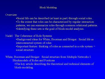
• Overview
• Social life can be described (at least in part)
  through social roles.
• To the extent that roles can be characterized by
  regular interaction patterns, we can summarize
  roles through common relational patterns.
• Identifying these sets is the goal of block-model
  analyses.
• Nadel The Coherence of Role Systems
• Background ideas for White, Boorman and Brieger.
  Social life as interconnected system of roles
• Important feature thinking of roles as connected
  in a role system social structure
• White, Boorman and Breiger Social structure
  from Multiple Networks I. Blockmodels of Roles
  and Positions
• The key article describing the theoretical and
  technical elements of block-modeling

2
Nadel The Coherence of Role Systems

• Elements of a Role
• Rights and obligations with respect to other
  people or classes of people
• Roles require a role compliment another person
  who the role-occupant acts with respect to
• Examples
• Parent - child, Teacher - student, Lover -
  lover, Friend - Friend, Husband - Wife, etc.
• Nadel (Following functional anthropologists and
  sociologists) defines logical types of roles,
  and then examines how they can be linked together.

3
Nadel The Coherence of Role Systems
Nadel describes role patterns in the book. In
the chapter we read, he focuses on how these
various roles fit together to form a coherent
whole. Roles are collected in people through
the summation of roles Necessary Some roles
fit together necessarily. For example, the
expected interaction patterns of son-in-law are
implied through the joint roles of Husband and
Spouse-Parent Coincidental Some roles tend
to go together empirically, but they need not
(businessman club member, for example).
Distinguishing the two is a matter of
usefulness and judgement, but relates to social
substitutability. The distinction reverts to how
the system as a whole will be held together in
the face of changes in role occupants.
4
Nadel The Coherence of Role Systems
Given that roles can be identified as going
together is there a logic that underlies their
connection? Nadel uses a functional description
based on ascription and achievement
5
Nadel The Coherence of Role Systems
And he gives an example of a simple role system
Nadels task is to make sense of these roles, to
identify how they are interconnected to form a
system -- a coherent structure. This is a
difficult task to do analytically, as the
eventual failure of Parsonian functionalism shows.
6
White et al From logical role systems to
empirical social structures
With the fall of parsons and functionalism in the
late 60s, many of the ideas about social
structure and system were also tossed. White
et al demonstrate how we can understand social
structure as the intercalation of roles, without
the a priori logical categories. Start with some
basic ideas of what a role is An exchange of
something (support, ideas, commands, etc) between
actors. Thus, we might represent a family as
7
White et al From logical role systems to
empirical social structures
Start with some basic ideas of what a role is
An exchange of something (support, ideas,
commands, etc) between actors. Thus, we might
represent a family as
H
W
C
C
C
Provides food for
(and there are, of course, many other relations
inside the family)
8
White et al From logical role systems to
empirical social structures
The key idea, is that we can express a role
through a relation (or set of relations) and thus
a social system by the inventory of roles. If
roles equate to positions in an exchange system,
then we need only identify particular aspects of
a position. But what aspect? Structural
Equivalence
Two actors are structurally equivalent if they
have the same types of ties to the same people.
9
Structural Equivalence
A single relation
10
Structural Equivalence
Graph reduced to positions
11
Alternative notions of equivalence
Instead of exact same ties to exact same alters,
you look for nodes with similar ties to similar
types of alters
12
Blockmodeling basic steps
In any positional analysis, there are 4 basic
steps 1) Identify a definition of
equivalence 2) Measure the degree to which pairs
of actors are equivalent 3) Develop a
representation of the equivalencies 4) Assess
the adequacy of the representation
13
1) Identify a definition of equivalence
Structural Equivalence Two actors are
equivalent if they have the same type of ties to
the same people.
14
1) Identify a definition of equivalence
Automorphic Equivalence Actors occupy
indistinguishable structural locations in the
network. That is, that they are in isomorphic
positions in the network. Two graphs are
isomorphic if there is some mapping of nodes to
positions that equates the two. For example, all
030T triads are isomorphic. A graph is
automorphic, if there are patterns internal to
the graph that are equated (if the mapping goes
from the set of nodes in the graph to other nodes
in the graph). In general, automorphically
equivalent nodes are equivalent with respect to
all graph theoretic properties (I.e. degree,
number of people reachable, centrality, etc.)
15
Automorphic Equivalence
16
1) Identify a definition of equivalence
Regular Equivalence Regular equivalence does
not require actors to have identical ties to
identical actors or to be structurally
indistinguishable. Actors who are regularly
equivalent have identical ties to and from
equivalent actors. If actors i and j are
regularly equivalent, then for all relations and
for all actors, if i k, then there exists
some actor l such that j l and k is regularly
equivalent to l.
17
Regular Equivalence
There may be multiple regular equivalence
partitions in a network, and thus we tend to want
to find the maximal regular equivalence position,
the one with the fewest positions.
18
Role or Local Equivalence While most
equivalence measures focus on position within the
full network, some measures focus only on the
patters within the local tie neighborhood. These
have been called local role equivalence. In
the example weve been using, they revert to
automorphic equivalence
Note that Structurally equivalent actors are
automorphically equivalent, Automorphically
equivalent actors are regularly
equivalent. Structurally equivalent and
automorphically equivalent actors are role
equivalent In practice, we tend to ignore some
of these fine distinctions, as they get blurred
quickly once we have to operationalize them in
real graphs. It turns out that few people are
ever exactly equivalent, and thus we approximate
the links between the types. In all cases, the
procedure can work over multiple relations
simultaneously. The process of identifying
positions is called blockmodeling, and requires
identifying a measure of similarity among nodes.
19
Blockmodeling is the process of identifying these
types of positions. A block is a section of the
adjacency matrix - a group of people.
0 1 1 1 0 0 0 0 0 0 0 0 0 0 1 0 0 0 1 1 0 0 0 0 0
0 0 0 1 0 0 1 0 0 1 1 1 1 0 0 0 0 1 0 1 0 0 0 1 1
1 1 0 0 0 0 0 1 0 0 0 1 0 0 0 0 1 1 1 1 0 1 0 0 1
0 0 0 0 0 1 1 1 1 0 0 1 1 0 0 0 0 0 0 0 0 0 0 0 0
1 1 0 0 0 0 0 0 0 0 0 0 0 0 1 1 0 0 0 0 0 0 0 0 0
0 0 0 1 1 0 0 0 0 0 0 0 0 0 0 0 0 0 0 1 1 0 0 0 0
0 0 0 0 0 0 0 0 1 1 0 0 0 0 0 0 0 0 0 0 0 0 1 1 0
0 0 0 0 0 0 0 0 0 0 0 1 1 0 0 0 0 0 0 0 0
Here I have blocked structurally equivalent actors
20
Once you block the matrix, reduce it, based on
the number of ties in the cell of interest. The
key values are a zero block (no ties) and a
one-block (all ties present)
1 2 3 4 5 6 1 0 1 1 0 0 0 2 1 0 0 1 0 0 3 1 0 1
0 1 0 4 0 1 0 1 0 1 5 0 0 1 0 0 0 6 0 0 0 1 0 0
1
2
3
4
5
6
1
. 1 1 1 0 0 0 0 0 0 0 0 0 0 1 . 0 0 1 1 0 0 0 0 0
0 0 0 1 0 . 1 0 0 1 1 1 1 0 0 0 0 1 0 1 . 0 0 1 1
1 1 0 0 0 0 0 1 0 0 . 1 0 0 0 0 1 1 1 1 0 1 0 0 1
. 0 0 0 0 1 1 1 1 0 0 1 1 0 0 . 0 0 0 0 0 0 0 0 0
1 1 0 0 0 . 0 0 0 0 0 0 0 0 1 1 0 0 0 0 . 0 0 0 0
0 0 0 1 1 0 0 0 0 0 . 0 0 0 0 0 0 0 0 1 1 0 0 0 0
. 0 0 0 0 0 0 0 1 1 0 0 0 0 0 . 0 0 0 0 0 0 1 1 0
0 0 0 0 0 . 0 0 0 0 0 1 1 0 0 0 0 0 0 0 .
2
3
4
5
6
Structural equivalence thus generates 6 positions
in the network
21
Once you partition the matrix, reduce it
. 1 1 1 0 0 0 0 0 0 0 0 0 0 1 . 0 0 1 1 0 0 0 0 0
0 0 0 1 0 . 1 0 0 1 1 1 1 0 0 0 0 1 0 1 . 0 0 1 1
1 1 0 0 0 0 0 1 0 0 . 1 0 0 0 0 1 1 1 1 0 1 0 0 1
. 0 0 0 0 1 1 1 1 0 0 1 1 0 0 . 0 0 0 0 0 0 0 0 0
1 1 0 0 0 . 0 0 0 0 0 0 0 0 1 1 0 0 0 0 . 0 0 0 0
0 0 0 1 1 0 0 0 0 0 . 0 0 0 0 0 0 0 0 1 1 0 0 0 0
. 0 0 0 0 0 0 0 1 1 0 0 0 0 0 . 0 0 0 0 0 0 1 1 0
0 0 0 0 0 . 0 0 0 0 0 1 1 0 0 0 0 0 0 0 .
1 2 3 1 1 1 0 2 1 1 1 3 0 1 0
1
2
3
Regular equivalence
(here I placed a one in the image matrix if there
were any ties in the ij block)
22
To get a block model, you have to measure the
similarity between each pair. If two actors are
structurally equivalent, then they will have
exactly similar patterns of ties to other people.
Consider the example again
C and D match on 12 other people
1
2
3
4
5
6
C D Match 1 1 1 0 0 1 . 1 0 1 . 0 0
0 1 0 0 1 1 1 1 1 1 1 1 1 1 1 1
1 0 0 1 0 0 1 0 0 1 0 0 1 Sum 12
1
. 1 1 1 0 0 0 0 0 0 0 0 0 0 1 . 0 0 1 1 0 0 0 0 0
0 0 0 1 0 . 1 0 0 1 1 1 1 0 0 0 0 1 0 1 . 0 0 1 1
1 1 0 0 0 0 0 1 0 0 . 1 0 0 0 0 1 1 1 1 0 1 0 0 1
. 0 0 0 0 1 1 1 1 0 0 1 1 0 0 . 0 0 0 0 0 0 0 0 0
1 1 0 0 0 . 0 0 0 0 0 0 0 0 1 1 0 0 0 0 . 0 0 0 0
0 0 0 1 1 0 0 0 0 0 . 0 0 0 0 0 0 0 0 1 1 0 0 0 0
. 0 0 0 0 0 0 0 1 1 0 0 0 0 0 . 0 0 0 0 0 0 1 1 0
0 0 0 0 0 . 0 0 0 0 0 1 1 0 0 0 0 0 0 0 .
2
3
4
5
6
23
If the model is going to be based on asymmetric
or multiple relations, you simply stack the
various relations
Stacked
Romance 0 1 0 0 0 1 0 0 0 0 0 0 0 0 0 0 0 0 0 0 0
0 0 0 0
0 1 0 0 0 1 0 0 0 0 0 0 0 0 0 0 0 0 0 0 0 0 0 0 0
H
W
0 0 1 1 1 0 0 1 1 1 0 0 0 0 0 0 0 0 0 0 0 0 0 0 0
Feeds 0 0 1 1 1 0 0 1 1 1 0 0 0 0 0 0 0 0 0 0 0 0
0 0 0
C
C
C
0 0 0 0 0 0 0 0 0 0 1 1 0 0 0 1 1 0 0 0 1 1 0 0 0
Romantic Love
Provides food for
Bicker 0 0 0 0 0 0 0 0 0 0 0 0 0 1 1 0 0 1 0 0 0
0 1 1 0
Bickers with
0 0 0 0 0 0 0 0 0 0 0 0 0 1 1 0 0 1 0 1 0 0 1 1 0
24
For the entire matrix, we get
0 8 7 7 5 5 11 11 11 11 7 7 7 7 8 0
5 5 7 7 7 7 7 7 11 11 11 11 7 5 0 12 0
0 8 8 8 8 4 4 4 4 7 5 12 0 0 0 8
8 8 8 4 4 4 4 5 7 0 0 0 12 4 4 4 4
8 8 8 8 5 7 0 0 12 0 4 4 4 4 8 8
8 8 11 7 8 8 4 4 0 12 12 12 8 8 8 8 11
7 8 8 4 4 12 0 12 12 8 8 8 8 11 7 8
8 4 4 12 12 0 12 8 8 8 8 11 7 8 8 4 4
12 12 12 0 8 8 8 8 7 11 4 4 8 8 8 8
8 8 0 12 12 12 7 11 4 4 8 8 8 8 8 8 12
0 12 12 7 11 4 4 8 8 8 8 8 8 12 12 0
12 7 11 4 4 8 8 8 8 8 8 12 12 12 0
(number of agreements for each ij pair)
25
The metric used to measure structural equivalence
by White, Boorman and Brieger is the correlation
between each nodes set of ties. For the
example, this would be
1.00 -0.20 0.08 0.08 -0.19 -0.19 0.77 0.77
0.77 0.77 -0.26 -0.26 -0.26 -0.26 -0.20 1.00
-0.19 -0.19 0.08 0.08 -0.26 -0.26 -0.26 -0.26
0.77 0.77 0.77 0.77 0.08 -0.19 1.00 1.00
-1.00 -1.00 0.36 0.36 0.36 0.36 -0.45 -0.45
-0.45 -0.45 0.08 -0.19 1.00 1.00 -1.00 -1.00
0.36 0.36 0.36 0.36 -0.45 -0.45 -0.45
-0.45 -0.19 0.08 -1.00 -1.00 1.00 1.00 -0.45
-0.45 -0.45 -0.45 0.36 0.36 0.36 0.36 -0.19
0.08 -1.00 -1.00 1.00 1.00 -0.45 -0.45 -0.45
-0.45 0.36 0.36 0.36 0.36 0.77 -0.26 0.36
0.36 -0.45 -0.45 1.00 1.00 1.00 1.00 -0.20
-0.20 -0.20 -0.20 0.77 -0.26 0.36 0.36 -0.45
-0.45 1.00 1.00 1.00 1.00 -0.20 -0.20 -0.20
-0.20 0.77 -0.26 0.36 0.36 -0.45 -0.45 1.00
1.00 1.00 1.00 -0.20 -0.20 -0.20 -0.20 0.77
-0.26 0.36 0.36 -0.45 -0.45 1.00 1.00 1.00
1.00 -0.20 -0.20 -0.20 -0.20 -0.26 0.77 -0.45
-0.45 0.36 0.36 -0.20 -0.20 -0.20 -0.20 1.00
1.00 1.00 1.00 -0.26 0.77 -0.45 -0.45 0.36
0.36 -0.20 -0.20 -0.20 -0.20 1.00 1.00 1.00
1.00 -0.26 0.77 -0.45 -0.45 0.36 0.36 -0.20
-0.20 -0.20 -0.20 1.00 1.00 1.00 1.00 -0.26
0.77 -0.45 -0.45 0.36 0.36 -0.20 -0.20 -0.20
-0.20 1.00 1.00 1.00 1.00
Another common metric is the Euclidean distance
between pairs of actors, which you then use in a
standard cluster analysis.
26
The initial method for finding structurally
equivalent positions was CONCOR, the CONvergence
of iterated CORrelations.
Concor iteration 1
1.00 -.77 0.55 0.55 -.57 -.57 0.95 0.95 0.95 0.95
-.75 -.75 -.75 -.75 -.77 1.00 -.57 -.57 0.55 0.55
-.75 -.75 -.75 -.75 0.95 0.95 0.95 0.95 0.55 -.57
1.00 1.00 -1.0 -1.0 0.73 0.73 0.73 0.73 -.75 -.75
-.75 -.75 0.55 -.57 1.00 1.00 -1.0 -1.0 0.73 0.73
0.73 0.73 -.75 -.75 -.75 -.75 -.57 0.55 -1.0 -1.0
1.00 1.00 -.75 -.75 -.75 -.75 0.73 0.73 0.73
0.73 -.57 0.55 -1.0 -1.0 1.00 1.00 -.75 -.75 -.75
-.75 0.73 0.73 0.73 0.73 0.95 -.75 0.73 0.73 -.75
-.75 1.00 1.00 1.00 1.00 -.77 -.77 -.77 -.77 0.95
-.75 0.73 0.73 -.75 -.75 1.00 1.00 1.00 1.00 -.77
-.77 -.77 -.77 0.95 -.75 0.73 0.73 -.75 -.75 1.00
1.00 1.00 1.00 -.77 -.77 -.77 -.77 0.95 -.75 0.73
0.73 -.75 -.75 1.00 1.00 1.00 1.00 -.77 -.77 -.77
-.77 -.75 0.95 -.75 -.75 0.73 0.73 -.77 -.77 -.77
-.77 1.00 1.00 1.00 1.00 -.75 0.95 -.75 -.75 0.73
0.73 -.77 -.77 -.77 -.77 1.00 1.00 1.00 1.00 -.75
0.95 -.75 -.75 0.73 0.73 -.77 -.77 -.77 -.77 1.00
1.00 1.00 1.00 -.75 0.95 -.75 -.75 0.73 0.73 -.77
-.77 -.77 -.77 1.00 1.00 1.00 1.00
27
The initial method for finding structurally
equivalent positions was CONCOR, the CONvergence
of iterated CORrelations.
Concor iteration 2
1.00 -.99 0.94 0.94 -.94 -.94 0.99 0.99 0.99 0.99
-.99 -.99 -.99 -.99 -.99 1.00 -.94 -.94 0.94 0.94
-.99 -.99 -.99 -.99 0.99 0.99 0.99 0.99 0.94 -.94
1.00 1.00 -1.0 -1.0 0.97 0.97 0.97 0.97 -.97 -.97
-.97 -.97 0.94 -.94 1.00 1.00 -1.0 -1.0 0.97 0.97
0.97 0.97 -.97 -.97 -.97 -.97 -.94 0.94 -1.0 -1.0
1.00 1.00 -.97 -.97 -.97 -.97 0.97 0.97 0.97
0.97 -.94 0.94 -1.0 -1.0 1.00 1.00 -.97 -.97 -.97
-.97 0.97 0.97 0.97 0.97 0.99 -.99 0.97 0.97 -.97
-.97 1.00 1.00 1.00 1.00 -.99 -.99 -.99 -.99 0.99
-.99 0.97 0.97 -.97 -.97 1.00 1.00 1.00 1.00 -.99
-.99 -.99 -.99 0.99 -.99 0.97 0.97 -.97 -.97 1.00
1.00 1.00 1.00 -.99 -.99 -.99 -.99 0.99 -.99 0.97
0.97 -.97 -.97 1.00 1.00 1.00 1.00 -.99 -.99 -.99
-.99 -.99 0.99 -.97 -.97 0.97 0.97 -.99 -.99 -.99
-.99 1.00 1.00 1.00 1.00 -.99 0.99 -.97 -.97 0.97
0.97 -.99 -.99 -.99 -.99 1.00 1.00 1.00 1.00 -.99
0.99 -.97 -.97 0.97 0.97 -.99 -.99 -.99 -.99 1.00
1.00 1.00 1.00 -.99 0.99 -.97 -.97 0.97 0.97 -.99
-.99 -.99 -.99 1.00 1.00 1.00 1.00
28
The initial method for finding structurally
equivalent positions was CONCOR, the CONvergence
of iterated CORrelations.
Concor iteration 3
1.00 -1.0 1.00 1.00 -1.0 -1.0 1.00 1.00 1.00 1.00
-1.0 -1.0 -1.0 -1.0 -1.0 1.00 -1.0 -1.0 1.00 1.00
-1.0 -1.0 -1.0 -1.0 1.00 1.00 1.00 1.00 1.00 -1.0
1.00 1.00 -1.0 -1.0 1.00 1.00 1.00 1.00 -1.0 -1.0
-1.0 -1.0 1.00 -1.0 1.00 1.00 -1.0 -1.0 1.00 1.00
1.00 1.00 -1.0 -1.0 -1.0 -1.0 -1.0 1.00 -1.0 -1.0
1.00 1.00 -1.0 -1.0 -1.0 -1.0 1.00 1.00 1.00
1.00 -1.0 1.00 -1.0 -1.0 1.00 1.00 -1.0 -1.0 -1.0
-1.0 1.00 1.00 1.00 1.00 1.00 -1.0 1.00 1.00 -1.0
-1.0 1.00 1.00 1.00 1.00 -1.0 -1.0 -1.0 -1.0 1.00
-1.0 1.00 1.00 -1.0 -1.0 1.00 1.00 1.00 1.00 -1.0
-1.0 -1.0 -1.0 1.00 -1.0 1.00 1.00 -1.0 -1.0 1.00
1.00 1.00 1.00 -1.0 -1.0 -1.0 -1.0 1.00 -1.0 1.00
1.00 -1.0 -1.0 1.00 1.00 1.00 1.00 -1.0 -1.0 -1.0
-1.0 -1.0 1.00 -1.0 -1.0 1.00 1.00 -1.0 -1.0 -1.0
-1.0 1.00 1.00 1.00 1.00 -1.0 1.00 -1.0 -1.0 1.00
1.00 -1.0 -1.0 -1.0 -1.0 1.00 1.00 1.00 1.00 -1.0
1.00 -1.0 -1.0 1.00 1.00 -1.0 -1.0 -1.0 -1.0 1.00
1.00 1.00 1.00 -1.0 1.00 -1.0 -1.0 1.00 1.00 -1.0
-1.0 -1.0 -1.0 1.00 1.00 1.00 1.00
29
The initial method for finding structurally
equivalent positions was CONCOR, the CONvergence
of iterated CORrelations.
Concor iteration 3
1.00 1.00 1.00 1.00 1.00 1.00 1.00 -1.0 -1.0 -1.0
-1.0 -1.0 -1.0 -1.0 1.00 1.00 1.00 1.00 1.00 1.00
1.00 -1.0 -1.0 -1.0 -1.0 -1.0 -1.0 -1.0 1.00 1.00
1.00 1.00 1.00 1.00 1.00 -1.0 -1.0 -1.0 -1.0 -1.0
-1.0 -1.0 1.00 1.00 1.00 1.00 1.00 1.00 1.00 -1.0
-1.0 -1.0 -1.0 -1.0 -1.0 -1.0 1.00 1.00 1.00 1.00
1.00 1.00 1.00 -1.0 -1.0 -1.0 -1.0 -1.0 -1.0
-1.0 1.00 1.00 1.00 1.00 1.00 1.00 1.00 -1.0 -1.0
-1.0 -1.0 -1.0 -1.0 -1.0 1.00 1.00 1.00 1.00 1.00
1.00 1.00 -1.0 -1.0 -1.0 -1.0 -1.0 -1.0 -1.0 -1.0
-1.0 -1.0 -1.0 -1.0 -1.0 -1.0 1.00 1.00 1.00 1.00
1.00 1.00 1.00 -1.0 -1.0 -1.0 -1.0 -1.0 -1.0 -1.0
1.00 1.00 1.00 1.00 1.00 1.00 1.00 -1.0 -1.0 -1.0
-1.0 -1.0 -1.0 -1.0 1.00 1.00 1.00 1.00 1.00 1.00
1.00 -1.0 -1.0 -1.0 -1.0 -1.0 -1.0 -1.0 1.00 1.00
1.00 1.00 1.00 1.00 1.00 -1.0 -1.0 -1.0 -1.0 -1.0
-1.0 -1.0 1.00 1.00 1.00 1.00 1.00 1.00 1.00 -1.0
-1.0 -1.0 -1.0 -1.0 -1.0 -1.0 1.00 1.00 1.00 1.00
1.00 1.00 1.00 -1.0 -1.0 -1.0 -1.0 -1.0 -1.0 -1.0
1.00 1.00 1.00 1.00 1.00 1.00 1.00
1 3 4 7 8 9 10 2 5 6 11 12 13 14
30
Repeat the process on the resulting 1-blocks
until you have reached structural equivalent
blocks
Because CONCOR splits every sub-group into two
groups, you get a partition tree that looks
something like this
31
Automorphic and Regular equivalence are more
difficult to find, and require iteratively
searching over possible class assignments for
sets that have the same graph theoretic patterns.
Usually start with a set of nodes defined as
similar on a number of network measures, then
look within these classes for automorphic
equivalence classes. A theoretically appealing
method for finding structures that are very
similar to regular equivalence, role equivalence,
uses the triad census. Each node is involved in
(n-1)(n-2)/2 triads, and occupies a particular
position in each of these triads. These
positions are summarized in the following figure
32
Triadic Position Census 36 Positions within 16
Directed Triads
Indicates the position.
33
Triadic Position Census 40 Positions within all
mutual ties but two types of relations
34
36 36 10 10 10 10 43 43 43 43 43 43 43 43 0 0
0 0 0 0 0 0 0 0 0 0 0 0 0 0 0 0 0
0 0 0 0 0 0 0 0 0 0 0 0 0 0 0 0
0 0 0 0 0 0 0 20 20 41 41 41 41 14 14 14 14
14 14 14 14 9 9 11 11 11 11 12 12 12 12 12 12
12 12 0 0 0 0 0 0 0 0 0 0 0 0 0 0
0 0 0 0 0 0 0 0 0 0 0 0 0 0 0 0 0
0 0 0 0 0 0 0 0 0 0 0 0 0 0 0 0
0 0 0 0 0 0 0 0 0 0 0 0 0 0 0 0 0
0 0 0 0 0 0 0 0 0 0 0 0 0 0 0 0
0 0 0 0 0 0 0 0 0 0 0 0 0 0 0 0 0
0 0 0 0 0 0 0 0 0 0 0 0 0 0 0 0
0 0 0 0 0 0 0 0 0 0 0 0 0 0 0 0 0
0 0 0 0 0 0 0 0 0 0 0 0 0 0 0 0
0 0 0 0 0 0 0 0 0 0 0 0 0 0 0 0 0
0 0 0 0 0 0 0 0 0 0 0 0 0 0 0 0
0 0 0 0 0 0 0 0 0 0 0 0 0 0 0 0
0 0 0 0 0 0 0 0 0 0 0 0 0 0 0 0 0
0 0 0 0 0 0 0 0 0 0 0 0 0 0 0 0
0 0 0 0 0 0 0 0 0 0 10 10 1 1 1 1 8
8 8 8 8 8 8 8 2 2 10 10 10 10 0 0 0
0 0 0 0 0 0 0 0 0 0 0 0 0 0 0 0 0
0 0 0 0 0 0 0 0 0 0 0 0 0 0 0 0
0 0 0 0 0 0 0 0 0 0 0 0 0 0 0 0 0
0 0 0 0 0 0 0 0 0 0 0 0 0 0 0 0
0 0 0 0 0 0 0 0 0 0 0 0 0 0 0 0 0
0 0 0 0 0 0 0 0 0 0 0 0 0 0 0 0
0 0 0 0 0 0 0 0 0 0 0 0 0 0 0 0 0
0 0 0 0 0 0 0 0 0 0 0 0 0 0 0 0
0 0 0 0 0 0 0 0 0 0 0 0 0 1 1 5 5
5 5 1 1 1 1 1 1 1 1
Triad position vectors for the example network,
resulting in 3 positions
35
Correlating each persons triad position vector
with each other persons results in the following
table, which clearly shows the positions that are
equivalent
1.00 1.00 0.64 0.64 0.64 0.64 0.98 0.98 0.98 0.98
0.98 0.98 0.98 0.98 1.00 1.00 0.64 0.64 0.64 0.64
0.98 0.98 0.98 0.98 0.98 0.98 0.98 0.98 0.64 0.64
1.00 1.00 1.00 1.00 0.50 0.50 0.50 0.50 0.50 0.50
0.50 0.50 0.64 0.64 1.00 1.00 1.00 1.00 0.50 0.50
0.50 0.50 0.50 0.50 0.50 0.50 0.64 0.64 1.00 1.00
1.00 1.00 0.50 0.50 0.50 0.50 0.50 0.50 0.50
0.50 0.64 0.64 1.00 1.00 1.00 1.00 0.50 0.50 0.50
0.50 0.50 0.50 0.50 0.50 0.98 0.98 0.50 0.50 0.50
0.50 1.00 1.00 1.00 1.00 1.00 1.00 1.00 1.00 0.98
0.98 0.50 0.50 0.50 0.50 1.00 1.00 1.00 1.00 1.00
1.00 1.00 1.00 0.98 0.98 0.50 0.50 0.50 0.50 1.00
1.00 1.00 1.00 1.00 1.00 1.00 1.00 0.98 0.98 0.50
0.50 0.50 0.50 1.00 1.00 1.00 1.00 1.00 1.00 1.00
1.00 0.98 0.98 0.50 0.50 0.50 0.50 1.00 1.00 1.00
1.00 1.00 1.00 1.00 1.00 0.98 0.98 0.50 0.50 0.50
0.50 1.00 1.00 1.00 1.00 1.00 1.00 1.00 1.00 0.98
0.98 0.50 0.50 0.50 0.50 1.00 1.00 1.00 1.00 1.00
1.00 1.00 1.00 0.98 0.98 0.50 0.50 0.50 0.50 1.00
1.00 1.00 1.00 1.00 1.00 1.00 1.00
36
Moving from a similarity/distance matrix to a
blockmodel number of groups and determining
blocks An important decision in an analysis
using CONCOR is how fine the partition should be
in other words, when should one stop splitting
positions? Theory and the interpretability of
the solution are the primary consideration in
deciding how many positions to produce. (WF,
p.378) In defining positions of actors, the
trick is to choose the point along the series
that gives a useful and interpretable partition
of the actors into equivalence classes. (WF
p.383)
37
Example Most common block structures identified
in schools
38
Once you have decided on a number of blocks, you
need to determine what counts as a one block or
a zero block. Usually this is a some
function of the density of the resulting
block. General rules Fat Fit Only put a one
in blocks with all ones in the adjacency
matrix Lean Fit Put a zero if all the cells
are zero, else put a one Density fit If the
average value of the cell is above a certain
cutoff. White, Boorman and Breiger used a lean
fit (zeroblock) rule for the examples in their
paper
39
An example White et al, figure 1. Biomedical
Specialty data
40
White et al, figure 3. Biomedical Specialty data
Key to structure lies in zero blocks
41
The foundation of the block model rests on a set
of 16 two-position blocks. White et al claim
these are the tools you can use to interpret the
role system
42
Changes over time. Two arguments
a) that stable structures develop b) that the
global structure might be stable, even if the
micro-structure is not.
(note that this is exactly what Bearman did with
the protest data)
43
Padget and Ansell Robust Action and the Rise of
the Medici

• Substantive question relates to effective
  state-building there is a tension between the
  need to control and organization and the ability
  to build the legitimacy and recognition required
  for reproduction. The distinction between boss
  and judge
• They use the marriage, economic and patronage
  networks
• Empirically, we know that the state oligarchy
  structure of Florence stabilized after the rise
  of the medici

44
Padget and Ansell Robust Action and the Rise of
the Medici
Medici Takeover
45
Padget and Ansell Robust Action and the Rise of
the Medici
The story they tell revolves around how Cosimo
deMedici was able to found a system that lasted
nearly 300 years, uniting a fractured political
structure. The paradox of Cosimo is that he
didnt seem to fit the role of a Machiavellian
leader as decisive and goal oriented. The answer
lies in the power resulting from robust action
embedded in a network of relations that gives
rise to no clear meaning and obligation, but
instead allows for multiple meanings and
obligations.
46
A real example Padget and Ansell Robust Action
and the Rise of the Medici Political Groups
in the attribute sense do not seem to exist, so
PA turn to the pattern of network relations
among families. This is the BLOCK reduction of
the full 92 family network.
47
An example Relations among Italian
families. Political and friendship ties
48
Recent models

• Recent work has generalized blockmodels in two
  directions
• Specific structural hypotheses
• example Core-periphery models (UCINET)
• Generalized blockmodeling based on particular
  relationship types
• Example Pat Doreians recent work the the PAJEK
  folks.

49
Core-periphery models
Borgatti SP and Everett M G (1999) Models of
core/periphery structures. Social Networks 21
375-395
50
Core-periphery models
Goal is to identify the partition that most
closely resembles
1 1 1 1
1 1 1 1
1 1 1 1
0 0 0 0
51
Generalized Block Models
The recent work on generalization focuses on the
patterns that determine a block. Instead of
focusing on just the density of a block, you can
identify a block as any set that has a particular
pattern of ties to any other set. Examples
include
52
Generalized Block Models
53
Compound Relations.
We can generalize the balance rule to multitudes
of compound relations
A friend of a friend is a friend
F x F F



The enemy of an enemy is a friend
E x E F
-
-

Use matrices for primary relations and matrix
multiplication for compounds
54
Compound Relations.
One of the most powerful tools in role analysis
involves looking at role systems through compound
relations. A compound relation is formed by
combining relations in single dimensions. The
best example of compound relations come from
kinship.
Nephew/Niece 0 0 0 0 1 0 0 1 1 0 0 0 0 0 0 0 0 0
0 0 0 0 0 0 0
Sibling 0 1 0 0 0 1 0 0 0 0 0 0 0 1 0 0 0 1 0 0 0
0 0 0 0
Child of 0 0 1 1 0 0 0 0 0 1 0 0 0 0 0 0 0 0 0
0 0 0 0 0 0

x
Sibling
Child of
S?C SC
55
An example of compound relations can be found in
WF. This role table catalogues the compounds
for two relations Is boss of and Is on the
same level as
56
Compound Relations.
Kinship networks form a foundation to social
structures. In the west, we have 2 primary
relations (Parent of, married to) and one
partitioning attribute (male or female).
So Parent of a Parent Grandparent Fathers
Father Paternal Grandfather Mothers Father
Maternal Grandfather Wifes Mothers Son
Brother-in-law Mothers Mothers sons son
Cousin (moms side) Quality The entire western
kinship structure can be decomposed into a set of
equations consisting of only Parent, Child, and
Gender. Quantity Given a fertility rate of 2
kids, the two-step kinship neighborhood would
have 26 people if the fertility rate were 3 the
same count goes up to 46.
2-steps includes aunts uncles, but not their
spouses.
57
Compound Relations.
The scientists second rule has to be to look for
regularity and exploit that for theory. Consider
as a good example, Harrison Whites Kinship model
58
Compound Relations.
The scientists second rule has to be to look for
regularity and exploit that for theory. Consider
as a good example, Harrison Whites Kinship model
Ego connects to any of these
59
Compound Relations.
Kinship networks form a foundation to social
structures. In China, we have the same 2
primary relations Parent of Married to But 3
partitioning attributes Gender Relative
Age Relational Order (1st wife, 2nd wife,
etc) This means that compounds we name as
equivalent (cousin, uncle) are named differently.
But, while westerners largely ignore gender
for anything other than final designation
(aunt/uncle, niece/nephew), Chinese kinship terms
are differentiated by parents line (maternal
aunt, maternal uncle, etc.). We know this
designation, but use it rarely.
60
Compound Relations.
2-steps includes aunts uncles, but not their
spouses.
61
Compound Relations.
Uncles
62
Compound Relations.
63
Compound Relations.
The Chinese extended family network for
normal relations westerners would recognize
includes 74 unique kinship terms. The same set
in the west has 28 different terms. Each of
these terms carries a different expected gift
exchange system at holidays and mourning attire
at death.
64
Compound Relations.
How has this system changed? Consider the
effects of the 1-child policy
With a fertility of 6, 2-step kinship nets would
have 166 people with 2 its 26. A full
implementation of 1-child removes the relative
age operator, erasing every kinship term
dependent on older or younger and means that
families play either in a maternal or a paternal
line, but not both.
Source Population research Bureau
65
Using Compound Relations theoretically
James Montgomery Patronage systems
66
Using Compound Relations theoretically
James Montgomery Patronage systems
67
Using Compound Relations theoretically
Other work on this general topic
68
Using Compound Relations theoretically
Other work on this general topic
69
Methods How to?

• The basic block model formation can be done in
  multiple ways
• Apply any of our group-finding algorithms to a
  role-based similarity matrix
• Here youre simply converting the conditions for
  equivalence to adjacency and solving for
  modularity. Requires either a community
  detection algorithm that uses valued ties or a
  binarization of the similarity matrix.
• Cluster node-level structural indices (get at
  regular/automorphic equivalence)
• - This is the evade correlate to SE from
  community detection cluster on a BUNCH of
  easy-to-calculate node-level network statistics
  and this gives you nodes that are equivalent
  (with respect to the measures you used!)

70
Methods How to?
The basic block model formation can be done in
multiple ways Role-specific algorithms
71
Methods How to?
The basic block model formation can be done in
multiple ways Role-specific algorithms
72
Methods How to?
The basic block model formation can be done in
multiple ways Role-specific algorithms
73
Methods How to?
The basic block model formation can be done in
multiple ways Role-specific algorithms
74
Methods How to?
The basic block model formation can be done in
multiple ways Role-specific algorithms
4-block structural equivalence in PAJEK
75
Methods How to?
The basic block model formation can be done in
multiple ways Role-specific algorithms
6-block regular equivalence in PAJEK
76
Methods How to?
Triad Structural Equivalence in SAS
77
Methods How to?
Triad Structural Equivalence in SAS
78
Methods How to?
Triad Structural Equivalence in SAS