
Linear, integer and goal programming - PowerPoint PPT Presentation
1 / 20
Title:
Linear, integer and goal programming
Description:
Linear, integer and goal programming - Basic formulations of problems ... a set of constraints that circumscribe the decision variables. ... – PowerPoint PPT presentation
Number of Views:90
Avg rating:3.0/5.0
Title: Linear, integer and goal programming
1
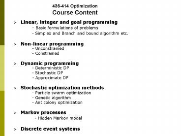
436-414 Optimization Course Content
- Linear, integer and goal programming
- - Basic formulations of problems
- - Simplex and Branch and bound algorithm etc.
- Non-linear programming - Unconstrained
- - Constrained
- Dynamic programming - Deterministic
DP - - Stochastic DP
- - Approximate DP
- Stochastic optimization methods
- - Particle swarm optimization
- - Genetic algorithm
- - Ant colony optimization
- Markov processes
- - Hidden Markov model
2
Linear and Integer Programming
Presented by Saman Halgamuge, University of
Melbourne Tutes and Projects by Kent Steer
3
Mathematical programming intro
- Mathematical programming (Planning/optimization
using mathematical models) to find the best
possible outcome - historical perspective most damage at the lowest
cost (_at_WW). - find an extreme (i.e., minimum or maximum) point
of a function, which satisfies a set of
constraints - A MP consists of
- a single objective function, representing either
a profit to be maximized or a cost to be
minimized, and - a set of constraints that circumscribe the
decision variables. - Applications of MP Layout design of a Micro
System, Number and the location of warehouses
needed, Optimal strategy development for
Greenhouse gas reduction, Optimal configuration
of a vehicle, production planning. - e.g. A company produces two varieties of a
product. Variety A has a profit per unit of 3.00
and variety B has a profit per unit of 2.00. - Demand for variety A is at most four units per
day. - Ten square meters of storage space is available
per day and one unit of A requires two square
meters whilst one unit of variety B requires one
square meter. - how many units of each product should the company
produce on a daily basis to maximize its profit? - This is a LP (Planning with Linear Models) - a
special case of MP
4
Linear programming a review
- Linear optimization or linear programming problem
has - Linear objective function
- Linear constrains (equal, less than or greater
than) - Continuous non-negative decision variables i.e.,
they can assume fractional values such as 3.2 - (non-negative integer under integer
programming)
5
Forms of LP problem
- LP problem is in the form of
maximize/
feasible region of the problem
where, -
vector of optimization variable -
objective function coefficients - constraint
coefficients - vector of right hand side of
constraints m - number of constraint equations,
n- number of variables
6
Graphical representation of the LP solution
- e.g. A manufacturing company produces two types
of products A and B. product A has a profit per
unit of 3.00 and variety B has a profit per unit
of 2.00. Demand for variety A is at most four
units per day. Production constraints are such
that at most 12 hours can be worked per day. 1
unit of A takes 1 hour to produce and 1 unit of B
takes 2 hours to produce. - 10 square meters of space is available
to store one day's production and 1 unit of
product A requires 2 square meters whilst 1 unit
of product B requires 1 square meter. - Formulate the problem of deciding
how much to produce per day in order to maximize
the daily profit as a linear program
Let, no of units of A produced no of
units of B produced Objective function
maximize Constraints Production
time Space Demand
Assume A and B are plastic containers. In using
LP, we must assume A and B do not have to be
produced in full and can take
fractions.
7
x2
14 12 10 8 6 4 2 0
feasible region
2
4
6
8
10
12
14
x1
8
The standard LP problem
find in order to minimize subject to
- We need a method to handle real life LPs with
many variables - We shall introduce a slack variable for each
inequality constraint - LP in the standard form has constraints converted
to equations and all variables are non negative - Before applying simplex algorithm, LP problem
must be converted into the standard form
9
Conversion to standard LP problem
- Maximization problem
- constants in the objective function
- Constraints containing lt
- add a positive variable (slack variable) to the
left hand side
10
Conversion to standard LP problem
- Constraints containing gt
- subtract a positive variable (slack variable)
from the left hand side - Negative values on the RHS of constrains
- All the constants of the r.h.s. must be positive
- Unrestricted variables
- Variable x with unrestricted sign is replaced by
two positive variables y1 and y2 as - if y1lty2, x is positive or if y1gty2, x is
negative.
11
- After converting to the standard form,
- If the number of constraint equations (m) is
equal to the number of variables (n), the
objective function is redundant and it is a
problem of solving a system of linear equations - The optimization is required when ngtm
- Simplex method is one of the popular techniques
for solving LP problems
mn2
mltn
12
Simplex algorithm
- It can be proved that the solution to the LP
problem is always on the boundary of the feasible
region which is a convex polygon - The solution is one of the extreme corners of
this polygon - Ideally, the solution can be found by checking
the objective value at each vertices - But checking all of them is computationally very
expensive. (Find the maximum bound for the number
of vertices?) - Simplex algorithm is a method which finds the
solution with a very few vertex checks.
13
Simplex algorithm
bfs basic feasible solution
bv basic variable
nbv non basic variable
14
For the next solution, Select the non-basic
variable to be basic As a rule of thumb, select
the non-basic variable in the objective function
with the largest negative (for the minimization
problem) coefficient since it may cause a largest
decrease in the objective value In this case, x1
is the candidate for the basic variable Then,
select the basic variable to become
non-basic Again, select the basic variable that
corresponds to the smallest ratio of the right
hand side of the constraint equations and the
coefficient of the newly found basic variables In
this case x1 is the new basic variable. 1st equ
12/1, 2nd equ 10/2, 3rd equ4, So, select s3 as
the new non-basic variable Then, basic x1,s1,s2
and non-basic x2, s3
e.g.
maximize
Step 1.) form the standard LP problem
minimize
Step 2.) find the starting bfs Slack variable
can be treated as basic variables Then,
basic by making non-basic
Note rewrite the problem such a way that the
objective function contains only non-basic
variables and each constraint equation contains
only one basic variable for the purpose of
easiness of the proceeding with the algorithm
15
For the 4th solution
minimize
3
s3 is the new basic variable s1 is the new
non-basic variable
Then basic x1,x2,s3 Nonbasic s1,s2
2nd Solution is,
For the 3rd solution
X2 has the largest negative coefficient So, x2 is
the next new basic variable. From the 2nd
constraint equation, s2 becomes the next new
non-basic variable Then basic x1,x2,s1 Nonbasic
s2,s3
Since all the coefficients of the objective
function are positive, this is the optimal
solution
16
Remarks
6 4 2
- The terminating condition of the algorithm is
that all the coefficients of the variables of the
objective function are positive. - Since the converged condition has been reached,
solution for the optimization problem is - Compare the sequence of the solutions and the
graphical representation of the problem.
x2
2
4
6
8
10
x1
12
17
Sensitivity analysis
- Consider the LP problem
- What is the effect on the optimal solution when
c and b are varied? - Sensitivity analysis gives insight into how LPs
parameters affect the optimal solution. - Sensitivity analysis also enables us to find the
new solution without solving the revised problem
with the changed parameters
18
Effect of change in an objective function
coefficient
6 4 2
In the previous example, what is the effect of
the current optimal basis, when the profit of
product A is changed
x2
d
2
4
6
8
10
x1
In order d to be still optimal when c is changed,
So, if the profit of product A is changed between
1 4 , the optimal solution, will remain
unchanged ( ). but the
overall profit ( ) will change.
19
Effect of change in a r.h.s. constraint
coefficients
6 4 2
similarly, what is the effect of the current
optimal basis (the current basic and non-basic
variables), when the available space is changed?
x2
(space constraint)
(work hour constraint)
2
4
6
8
10
x1
20
- The change of b shifts the space constraint
parallel to its current position - As long as the movement of the space constraint
line happens in between two red dashed lines (as
shown in figure), - the current basis remains optimal.
- the optimal solution occurs where the space and
work hour constraints intersects ? if
the solution to the optimization problem is
the solution of the two linear equations space
and work hour.
- By further analysis, we can see how much the
decision variables (x1,x2) are changed with the
change of b, i.e. how sensitive the decision
variables to change of b
Recommended
CrystalGraphics Presentations


