
Generating FullFactorial Models in Minitab - PowerPoint PPT Presentation
1 / 24
Title:
Generating FullFactorial Models in Minitab
Description:
smaller distances, but with only two reps, we'll press on! ... Set Pin Position to 0 (coded) which equates to 2 (actual: what you set in your design) ... – PowerPoint PPT presentation
Number of Views:77
Avg rating:3.0/5.0
Title: Generating FullFactorial Models in Minitab
1
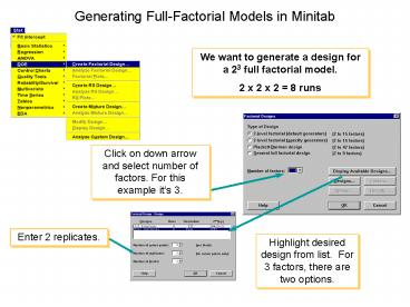
Generating Full-Factorial Models in Minitab
We want to generate a design for a 23 full
factorial model. 2 x 2 x 2 8 runs
Click on down arrow and select number of factors.
For this example its 3.
Enter 2 replicates.
Highlight desired design from list. For 3
factors, there are two options.
2
Generating Full-Factorial Models in Minitab
Click on Factors button
After selecting the design, you can name the
factors (Xs) and define their low and high values
3
Generating Full-Factorial Models in Minitab
After entering your factors, Click on the Options
button De-Select the Randomize runs
Then click OK twice
4
What Do You See
Notice Minitab gives you the values you need to
run your experimentnot 1 and 1.
Since we didnt randomize and we made
Start Angle factor C, we only need to change
start angle once.
It is recommended to RANDOMIZE YOUR EXPERIMENT
Notes 1) A new worksheet will be created for
the design. 2) The Minitab default is to
randomize the run order.
5
For our Design
6
Analyzing the Results of the DOE Step 9
Lets look at some graphs
7
Analyzing the Results of the DOE Step 9
Click on the double arrow button to transfer all
available terms into selected terms
Perform these steps in both setupMain Effects
Interactions
Make sure you have Distance in the Responses box
8
Analyzing the Results of the DOE Step 9
It looks like Start Angle and Pin Position had a
big effect on our Y--Distance
9
Analyzing the Results of the DOE Step 9
Since the lines are nearly parallel, the two-way
interactions will probably be insignificant
10
Analyzing the Results of the DOE Step 9
Go to StatgtDOEgtAnalyze Factorial Design
11
Analyzing the Results of the DOE Step 9
1. Put Distance in Responses
3. Then Pareto with Alpha 0.05
2. Click on Graphs
3. Click on these 3 Plots
4. Finally click Ok
12
Analyzing the Results of the DOE Step 9
1. Then click on Storage
3. Then Ok and Ok
2. Select Fits Residuals
13
Analyzing the Results of the DOE Step 9
These 3 graphs give you a good idea about whats
going on
14
Analyzing the Results of the DOE Steps 10 11
Steps 10 11 Plot Interpret the Residuals
- Residuals are the difference between the actual Y
value and the Y value predicted by the regression
equation. - Residuals should
- be randomly and normally distributed about a mean
of zero - not correlate with the predicted Y
- not exhibit trends over time (if data
chronological) - Stat gt DOE gt Analyze Factorial Design, Graphs
button - Select
- normal plot of residuals
- residuals against fits
- residuals against order
- Any trends or patterns in the residual plots
indicates inadequacies in the regression model,
such as missing Xs or nonlinear relationships.
15
Analyzing the Results of the DOE Steps 10 11
Lets look at each graph individually
16
Analyzing the Results of the DOE Steps 10 11
But first lets perform a Normality test on The
residuals by going to StatgtBasic
StatisticsgtNormality Test
In variable, select RESI1
Then click Ok
17
Analyzing the Results of the DOE Steps 10 11
P-value 0.497
Residuals Look normal
If residuals are not normal, your model may not
predict very well
18
Analyzing the Results of the DOE Steps 10 11
No trends in this graph
19
Analyzing the Results of the DOE Steps 10 11
This graph indicates there might be more
variability in the smaller distances, but with
only two reps, well press on!
20
Analyzing the Results of the DOE Step
12Examine the Factor Effects
Well keep Anything with A low P-value Lower
than 0.05
Since were keeping the 3-way interaction, we
need to include stop position in the model
21
Analyzing the Results of the DOE Step
12Examine the Factor Effects
Put 2-way interactions back in Available Terms
Go back in StatgtDOEgtAnalyze Factorial Design and
click on Terms, then remove the two-way
interactions
22
Step 13 Develop Prediction Models
Coefficients for the Coded model
Y 145.4 11.3A 0.7B 29.2C 1.31ABC
Coefficients for the Uncoded model
Y -339.4 9.4A 2.9B 2.9C
23
For the Coded Model
Y 145.4 11.3A 0.7B 29.2C 1.31ABC
- 145 145.4 11.3 (Pin Position) 0.7(Stop
Position) 29.2(Start Angle) 1.3(ABC) - Lets just arbitrarily set A B to some value
since they are discrete - Set Pin Position to 0 (coded) which equates to 2
(actual what you set in your design) - Stop Position at 1 (coded) which equates to 2
(actual what you set in your design) - Lets figure out Start Angle
- 145 145.4 11.3(0) 0.7(-1) 29.2 (Start
Angle) 1.31(0-1C) - 145 145.4 0 0.7 29.2(Start Angle) - 0
- 145 145.4 0.7 29.2(Start Angle)
- 0.3 29.2(Start Angle)
- 0.01 Start Angle
- Converting from the coded units
24
For the Un-coded Model
Y -339.4 9.4A 2.9B 2.9C 0.0ABC
- 145 -339.4 9.4 (Pin Position) 2.9(Stop
Position) 2.9(Start Angle) - Lets just arbitrarily set A B to some value
since they are discrete - Set Pin Position to 2
- Stop Position at 2
- Lets figure out Start Angle
- 145 -339.4 9.4(2) 2.9(2) 2.9(Start
Angle) - 145 -339.4 18.8 5.8 2.9(Start Angle)
- 497.4 2.9(Start Angle)
- 497.4 / 2.9 (Start Angle)
- 171.5 Start Angle