Lazy vs. Eager Learning

1
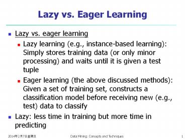
Lazy vs. Eager Learning

• Lazy vs. eager learning
• Lazy learning (e.g., instance-based learning)
  Simply stores training data (or only minor
  processing) and waits until it is given a test
  tuple
• Eager learning (the above discussed methods)
  Given a set of training set, constructs a
  classification model before receiving new (e.g.,
  test) data to classify
• Lazy less time in training but more time in
  predicting

2
Lazy Learner Instance-Based Methods

• Instance-based learning
• Store training examples and delay the processing
  (lazy evaluation) until a new instance must be
  classified
• Typical approaches
• k-nearest neighbor approach
• Instances represented as points in a Euclidean
  space.
• Locally weighted regression
• Constructs local approximation
• Case-based reasoning
• Uses symbolic representations and knowledge-based
  inference

3
The k-Nearest Neighbor Algorithm

• All instances correspond to points in the n-D
  space
• The nearest neighbor are defined in terms of
  Euclidean distance, dist(X1, X2)
• Target function could be discrete- or real-
  valued
• For discrete-valued, k-NN returns the most common
  value among the k training examples nearest to xq
• Vonoroi diagram the decision surface induced by
  1-NN for a typical set of training examples

.
_
_
_
.
_
.

.

.
_

xq
.
_

4
Discussion on the k-NN Algorithm

• k-NN for real-valued prediction for a given
  unknown tuple
• Returns the mean values of the k nearest
  neighbors
• Distance-weighted nearest neighbor algorithm
• Weight the contribution of each of the k
  neighbors according to their distance to the
  query xq
• Give greater weight to closer neighbors
• Robust to noisy data by averaging k-nearest
  neighbors
• Curse of dimensionality distance between
  neighbors could be dominated by irrelevant
  attributes
• To overcome it, elimination of the least relevant
  attributes

5
Genetic Algorithms (GA)

• Genetic Algorithm based on an analogy to
  biological evolution
• An initial population is created consisting of
  randomly generated rules
• Each rule is represented by a string of bits
• E.g., if A1 and A2 then C2 can be encoded as 100
  
• If an attribute has k gt 2 values, k bits can be
  used
• Based on the notion of survival of the fittest, a
  new population is formed to consist of the
  fittest rules and their offsprings
• The fitness of a rule is represented by its
  classification accuracy on a set of training
  examples
• Offsprings are generated by crossover and
  mutation
• The process continues until a population P
  evolves when each rule in P satisfies a
  prespecified threshold
• Slow but easily parallelizable

6
Rough Set Approach

• Rough sets are used to approximately or roughly
  define equivalent classes
• A rough set for a given class C is approximated
  by two sets a lower approximation (certain to be
  in C) and an upper approximation (cannot be
  described as not belonging to C)
• Finding the minimal subsets (reducts) of
  attributes for feature reduction is NP-hard but a
  discernibility matrix (which stores the
  differences between attribute values for each
  pair of data tuples) is used to reduce the
  computation intensity

7
Fuzzy Set Approaches

• Fuzzy logic uses truth values between 0.0 and 1.0
  to represent the degree of membership (such as
  using fuzzy membership graph)
• Attribute values are converted to fuzzy values
• e.g., income is mapped into the discrete
  categories low, medium, high with fuzzy values
  calculated
• For a given new sample, more than one fuzzy value
  may apply
• Each applicable rule contributes a vote for
  membership in the categories
• Typically, the truth values for each predicted
  category are summed, and these sums are combined

8
Classifier Accuracy Measures
C1 C2
C1 True positive False negative
C2 False positive True negative
classes buy_computer yes buy_computer no total recognition()
buy_computer yes 6954 46 7000 99.34
buy_computer no 412 2588 3000 86.27
total 7366 2634 10000 95.52

• Accuracy of a classifier M, acc(M) percentage of
  test set tuples that are correctly classified by
  the model M
• Error rate (misclassification rate) of M 1
  acc(M)
• Given m classes, CMi,j, an entry in a confusion
  matrix, indicates of tuples in class i that
  are labeled by the classifier as class j
• Alternative accuracy measures (e.g., for cancer
  diagnosis)
• sensitivity t-pos/pos / true
  positive recognition rate /
• specificity t-neg/neg / true
  negative recognition rate /
• precision t-pos/(t-pos f-pos)
• accuracy sensitivity pos/(pos neg)
  specificity neg/(pos neg)
• This model can also be used for cost-benefit
  analysis

9
Evaluating the Accuracy of a Classifier

• Holdout method
• Given data is randomly partitioned into two
  independent sets
• Training set (e.g., 2/3) for model construction
• Test set (e.g., 1/3) for accuracy estimation
• Cross-validation (k-fold, where k 10 is most
  popular)
• Randomly partition the data into k mutually
  exclusive subsets, each approximately equal size
• At i-th iteration, use Di as test set and others
  as training set
• Leave-one-out k folds where k of tuples, for
  small sized data

10
Evaluating the Accuracy of a Classifier or
Predictor (II)

• Bootstrap
• Works well with small data sets
• Samples the given training tuples uniformly with
  replacement
• i.e., each time a tuple is selected, it is
  equally likely to be selected again and re-added
  to the training set
• Several boostrap methods, and a common one is
  .632 boostrap
• Suppose we are given a data set of d tuples. The
  data set is sampled d times, with replacement,
  resulting in a training set of d samples. The
  data tuples that did not make it into the
  training set end up forming the test set. About
  63.2 of the original data will end up in the
  bootstrap, and the remaining 36.8 will form the
  test set (since (1 1/d)d e-1 0.368)
• Repeat the sampling procedue k times, overall
  accuracy of the model

11
Ensemble Methods Increasing the Accuracy

• Ensemble methods
• Use a combination of models to increase accuracy
• Combine a series of k learned models, M1, M2, ,
  Mk, with the aim of creating an improved model M
• Popular ensemble methods
• Bagging averaging the prediction over a
  collection of classifiers
• Boosting weighted vote with a collection of
  classifiers

12
Bagging Boostrap Aggregation

• Analogy Diagnosis based on multiple doctors
  majority vote
• Training
• Given a set D of d tuples, at each iteration i, a
  training set Di of d tuples is sampled with
  replacement from D (i.e., boostrap)
• A classifier model Mi is learned for each
  training set Di
• Classification classify an unknown sample X
• Each classifier Mi returns its class prediction
• The bagged classifier M counts the votes and
  assigns the class with the most votes to X
• Prediction can be applied to the prediction of
  continuous values by taking the average value of
  each prediction for a given test tuple
• Accuracy
• Often significant better than a single classifier
  derived from D
• For noise data not considerably worse, more
  robust
• Proved improved accuracy in prediction

13
Boosting

• Analogy Consult several doctors, based on a
  combination of weighted diagnosesweight assigned
  based on the previous diagnosis accuracy
• How boosting works?
• Weights are assigned to each training tuple
• A series of k classifiers is iteratively learned
• After a classifier Mi is learned, the weights are
  updated to allow the subsequent classifier, Mi1,
  to pay more attention to the training tuples that
  were misclassified by Mi
• The final M combines the votes of each
  individual classifier, where the weight of each
  classifier's vote is a function of its accuracy
• The boosting algorithm can be extended for the
  prediction of continuous values
• Comparing with bagging boosting tends to achieve
  greater accuracy, but it also risks overfitting
  the model to misclassified data

14
Adaboost (Freund and Schapire, 1997)

• Given a set of d class-labeled tuples, (X1, y1),
  , (Xd, yd)
• Initially, all the weights of tuples are set the
  same (1/d)
• Generate k classifiers in k rounds. At round i,
• Tuples from D are sampled (with replacement) to
  form a training set Di of the same size
• Each tuples chance of being selected is based on
  its weight
• A classification model Mi is derived from Di
• Its error rate is calculated using Di as a test
  set
• If a tuple is misclssified, its weight is
  increased, o.w. it is decreased
• Error rate err(Xj) is the misclassification
  error of tuple Xj. Classifier Mi error rate is
  the sum of the weights of the misclassified
  tuples
• The weight of classifier Mis vote is

15
Summary (I)

• Supervised learning
• Classification algorithms
• Accuracy measures
• Validation methods

16
Summary (II)

• Stratified k-fold cross-validation is a
  recommended method for accuracy estimation.
  Bagging and boosting can be used to increase
  overall accuracy by learning and combining a
  series of individual models.
• Significance tests and ROC curves are useful for
  model selection
• There have been numerous comparisons of the
  different classification and prediction methods,
  and the matter remains a research topic
• No single method has been found to be superior
  over all others for all data sets
• Issues such as accuracy, training time,
  robustness, interpretability, and scalability
  must be considered and can involve trade-offs,
  further complicating the quest for an overall
  superior method

17
References (1)

• C. Apte and S. Weiss. Data mining with decision
  trees and decision rules. Future Generation
  Computer Systems, 13, 1997.
• C. M. Bishop, Neural Networks for Pattern
  Recognition. Oxford University Press, 1995.
• L. Breiman, J. Friedman, R. Olshen, and C. Stone.
  Classification and Regression Trees. Wadsworth
  International Group, 1984.
• C. J. C. Burges. A Tutorial on Support Vector
  Machines for Pattern Recognition. Data Mining and
  Knowledge Discovery, 2(2) 121-168, 1998.
• P. K. Chan and S. J. Stolfo. Learning arbiter and
  combiner trees from partitioned data for scaling
  machine learning. KDD'95.
• W. Cohen. Fast effective rule induction.
  ICML'95.
• G. Cong, K.-L. Tan, A. K. H. Tung, and X. Xu.
  Mining top-k covering rule groups for gene
  expression data. SIGMOD'05.
• A. J. Dobson. An Introduction to Generalized
  Linear Models. Chapman and Hall, 1990.
• G. Dong and J. Li. Efficient mining of emerging
  patterns Discovering trends and differences.
  KDD'99.

18
References (2)

• R. O. Duda, P. E. Hart, and D. G. Stork. Pattern
  Classification, 2ed. John Wiley and Sons, 2001
• U. M. Fayyad. Branching on attribute values in
  decision tree generation. AAAI94.
• Y. Freund and R. E. Schapire. A
  decision-theoretic generalization of on-line
  learning and an application to boosting. J.
  Computer and System Sciences, 1997.
• J. Gehrke, R. Ramakrishnan, and V. Ganti.
  Rainforest A framework for fast decision tree
  construction of large datasets. VLDB98.
• J. Gehrke, V. Gant, R. Ramakrishnan, and W.-Y.
  Loh, BOAT -- Optimistic Decision Tree
  Construction. SIGMOD'99.
• T. Hastie, R. Tibshirani, and J. Friedman. The
  Elements of Statistical Learning Data Mining,
  Inference, and Prediction. Springer-Verlag,
  2001.
• D. Heckerman, D. Geiger, and D. M. Chickering.
  Learning Bayesian networks The combination of
  knowledge and statistical data. Machine Learning,
  1995.
• M. Kamber, L. Winstone, W. Gong, S. Cheng, and
  J. Han. Generalization and decision tree
  induction Efficient classification in data
  mining. RIDE'97.
• B. Liu, W. Hsu, and Y. Ma. Integrating
  Classification and Association Rule. KDD'98.
• W. Li, J. Han, and J. Pei, CMAR Accurate and
  Efficient Classification Based on Multiple
  Class-Association Rules, ICDM'01.

19
References (3)

• T.-S. Lim, W.-Y. Loh, and Y.-S. Shih. A
  comparison of prediction accuracy, complexity,
  and training time of thirty-three old and new
  classification algorithms. Machine Learning,
  2000.
• J. Magidson. The Chaid approach to segmentation
  modeling Chi-squared automatic interaction
  detection. In R. P. Bagozzi, editor, Advanced
  Methods of Marketing Research, Blackwell
  Business, 1994.
• M. Mehta, R. Agrawal, and J. Rissanen. SLIQ A
  fast scalable classifier for data mining.
  EDBT'96.
• T. M. Mitchell. Machine Learning. McGraw Hill,
  1997.
• S. K. Murthy, Automatic Construction of Decision
  Trees from Data A Multi-Disciplinary Survey,
  Data Mining and Knowledge Discovery 2(4)
  345-389, 1998
• J. R. Quinlan. Induction of decision trees.
  Machine Learning, 181-106, 1986.
• J. R. Quinlan and R. M. Cameron-Jones. FOIL A
  midterm report. ECML93.
• J. R. Quinlan. C4.5 Programs for Machine
  Learning. Morgan Kaufmann, 1993.
• J. R. Quinlan. Bagging, boosting, and c4.5.
  AAAI'96.

20
References (4)

• R. Rastogi and K. Shim. Public A decision tree
  classifier that integrates building and pruning.
  VLDB98.
• J. Shafer, R. Agrawal, and M. Mehta. SPRINT A
  scalable parallel classifier for data mining.
  VLDB96.
• J. W. Shavlik and T. G. Dietterich. Readings in
  Machine Learning. Morgan Kaufmann, 1990.
• P. Tan, M. Steinbach, and V. Kumar. Introduction
  to Data Mining. Addison Wesley, 2005.
• S. M. Weiss and C. A. Kulikowski. Computer
  Systems that Learn Classification and
  Prediction Methods from Statistics, Neural Nets,
  Machine Learning, and Expert Systems. Morgan
  Kaufman, 1991.
• S. M. Weiss and N. Indurkhya. Predictive Data
  Mining. Morgan Kaufmann, 1997.
• I. H. Witten and E. Frank. Data Mining Practical
  Machine Learning Tools and Techniques, 2ed.
  Morgan Kaufmann, 2005.
• X. Yin and J. Han. CPAR Classification based on
  predictive association rules. SDM'03
• H. Yu, J. Yang, and J. Han. Classifying large
  data sets using SVM with hierarchical clusters.
  KDD'03.