Transformation of stress components

1
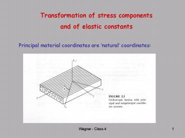
Transformation of stress components and of
elastic constants
Principal material coordinates are natural
coordinates
2
Sign convention
It is often necessary to know the stress-strain
relationships in non-principal coordinates
(off-axis) such as x and y. Therefore How do
we transform stress and strain? How do we
transform the elastic constants?
3
Transformation of stress components between
coordinate axes
This is obtained by writing a force balance
equation in a given direction. For example, in
the x direction
4
By repeating this, the complete set of stress
transformations in xy coordinates can be obtained
()
where c cosq and s sinq
And in the 12 system we have
with
5
Similarly, we have
()
Now, remember that for a 2-dimensional lamina in
its principal coordinates we showed that
()
(remember only 4 independent constants).
6
Then, substituting () into (), and then into
(), we find
7
and the components of the transformed reduced
stiffness matrix are as follows
(How many independent constants among these
transformed components?)
In terms of engineering constants, we have
8
EXAMPLES
Nylon-reinforced elastomer composite
9
Zinc (hexagonal symmetry)
Carbon AS4/epoxy composite
10
Anisotropy of bone (J. Biomechanics 1992)
11
Therefore, from the relationships
it is clear that we must know (and find ways to
measure and/or predict) the principal elastic
constants E1, E2, G12, n12 ! This is the topic
of micromechanics models
12
Micromechanics models for elastic constants

• Microstructural aspects
• The elastic constants can be measured through
  careful experiments. However, it is desirable to
  be able to reliably predict lamina properties as
  a function of constituent properties and
  geometric characteristics (such as fiber volume
  fraction and geometric packing characteristics).
• Thus we will be looking for a functional
  relationship of the following type

13
Typical transverse cross-sections of
unidirectional compositesComposites with low
volume fractions tend to have a random fiber
distribution, whereas with high volume fractions
the fibers tend to pack hexagonally.
Silicon carbide/glass ceramic,
fiber diameter 15 mm, Vf 0.40
Carbon/epoxy, fiber
diameter 8 mm, Vf 0.70
14
Expected volume fractions in composites using
representative area elements
NOTE - It is assumed that the fiber spacing (s)
and the fiber diameter (d) do not change along
the fiber length, so that area fractions volume
fractions
Max(Vf) _at_ sd Vf 0.907
Max(Vf) _at_ sd Vf 0.785
In practice, max(Vf) 0.5 0.8
15
Fiber content, matrix content, void content

• For n constituent materials we must have for
  volume fractions vi Vi/Vtot

In many cases this simply reduces to
For weight fractions wi Wi/Wtot, we have
16
(No Transcript)
17
Since weight (density)(volume), we obtain
immediately
thus, a Rule of Mixtures, which for 2-phase
composites becomes
And in terms of weight fractions instead of
volume fractions
The void fraction can be calculated from measured
weights (not fractions) and densities
18
Other structural aspects to be quantified
The fiber length distribution
19
The fiber orientation and the fiber orientation
distribution
20
The same formula may be used to calculate the
real depth of a hole from a (SEM) picture at an
angle
21
2. Elementary mechanics models
Longitudinal Youngs modulus - Assume an
isostrain situation (Voigt 1910) implicitely
perfect interfacial adhesion
Assuming linear elasticity for the fiber and
matrix
22
Assume Ac, Af, Am are the cross-sectional areas
of the composite, the fiber and the matrix. From
balancing the forces in the fiber direction, we
have
Therefore
and
Thus
(Voigt)
Also
23
Transverse Youngs modulus - Assume an isostress
situation (Reuss 1929)
In this case it is easily shown that
(Reuss)
24
Voigt bound
Reuss bound
25
A few remarks

• The longitudinal modulus is always greater than
  the transverse modulus
• The ratio E11/E22 may be considered as a measure
  of the degree of anisotropy (or orthotropy) of
  the lamina
• Poisson ratio n12 is also predicted by a rule of
  mixtures
• The shear modulus G12 is predicted by an inverse
  rule of mixtures
• Improved (tighter) bounds were developed by
  various authors (Hashin Shtrikman Hashin
  Rosen)

26
3. Semiempirical models

• The most successful semiempirical model is that
  of Halpin Tsai (1967)

where p represents composite moduli, for example
E11, E22, G12 or G23 pf and pm are the
corresponding fiber and matrix moduli. x is the
measure of the degree of reinforcement of the
matrix by the fibers, which depends on fiber
geometry and distribution, loading conditions,
etc. It is essentially a fitting factor.
27
These equations are quite accurate at low volume
fractions, a bit less so at higher volume
fractions. They have been modified to include the
maximum packing fraction. Specific values include
the following
Note finally that when x?0, the inverse rule of
mixtures is obtained, and when x?8, the direct
rule of mixtures is obtained.
28

• 1. INTRODUCTION GENERAL PRINCIPLES AND BASIC
  CONCEPTS
• Composites in the real world Classification of
  composites scale effects the role of
  interfacial area and adhesion three simple
  models for a-priori materials selection the role
  of defects Stress and strain thermodynamics of
  deformation and Hookes law anisotropy and
  elastic constants micromechanics models for
  elastic constants Lectures 1-2
• 2. MATERIALS FOR COMPOSITES FIBERS, MATRICES
• Types and physical properties of fibers
  flexibility and compressive behavior stochastic
  variability of strength Limits of fiber
  performance types and physical properties of
  matrices combining the phases residual thermal
  stresses Lectures 3-4
• 3. THE PRINCIPLES OF FIBER REINFORCEMENT
• Stress transfer The model of Cox The model of
  Kelly Tyson Other model Lectures 5-6
• 4. INTERFACES IN COMPOSITES
• Basic issues, wetting and contact angles,
  interfacial adhesion, the fragmentation
• phenomenon, microRaman spectroscopy,
  transcrystalline interfaces, Lectures 7-8
• 5. FRACTURE PHYSICS OF COMPOSITES
• Griffith theory of fracture, current models for
  idealized composites, stress concentration,
  simple mechanics of materials, micromechanics of
  composite strength, composite toughness Lectures
  9-11
• 6. DESIGN EXAMPLE
• A composite flywheel Lecture 12

29
CHAPTER 2 Materials for CompositesFibers and
matrices

• Types of Fiber Reinforcement
• Glass fibers
• Carbon or Graphite Fibers
• Aramid Fibers
• Polyethylene Fibers
• Rigid Rod Polymer Fibers
• Boron Fibers
• Silicon Carbide Fibers
• Other ceramic fibers
• Prospects for future reinforcement
• Self-Reinforcing Composites Molecular
  Reinforcement
• Natural Fiber Composites
• Carbon Nanotubes

30
Glass fibers

• Bulk glass tensile strength 0.7 to 1.4 GPa
• Fiber form from 3.5 to 5 GPa
• Isotropic and amorphous No crystalline order
• Used with epoxy and polyester mostly
• Susceptible to stress corrosion
• Poor fatigue resistance
• Good weather and chemical corrosion resistance
• 3D network, ionic and covalent bonds
• Sizing agent added after drawing
• Organosilane coupling agent X3SiR---matrix, X
  hydrolizes in presence of water to form silanol
  groups --- glass surface
• Density 2.54 g/cc
• Fine surface cracks leads to strength
  variability, size effects

31
Amorphous structure of glass
two dimensional representation of silica glass
network
modified network (Na2O added)
Each polyhedron can be seen to be a combination
of oxygen atoms around a silicon atom bonded
together by covalent bonds. The sodium ions form
ionic bonds with charged oxygen atoms and are not
linked directly to the network. The
three-dimensional network structure of glass
results in isotropic properties of glass fibers,
in contrast to those of carbon and Kevlar aramid
fibers which are anisotropic. The elastic modulus
of glass fibers measured along the fiber axis is
the same as that measured in the transverse
direction, a characteristic unique to glass
fibers.
32
Composition E Glass C Glass S
Glass SiO2 55.2 65.0 65.0 Al2O3 8.0 4.0 25.0 C
aO 18.7 14.0 - MgO 4.6 3.0 10.0 Na2O 0.3 8.5 0.3
K2O 0.2 - - B2O3 7.3 5.0 -
33

34
(No Transcript)
35
Sizing materials are normally coated on the
surface of glass fibers immediately after forming
as protection from mechanical damage. For glass
fibers intended for weaving, braiding or other
textile operations, the sizing usually consists
of a mixture of starch and a lubricant, which can
be removed from the fiber by burning after the
fibers have been processed into a textile
structure. For glass reinforcement used in
composites, the sizing usually contains a
coupling agent to bridge the fiber surface with
the resin matrix used in the composite. These
coupling agents are usually organosilanes with
the structure X3SiR, although sometimes titanate
and other chemical structures are used. The R
group may be able to react with a group in the
polymer of the matrix the X groups can hydrolyze
in the presence of water to form silanol groups
which can condense with the silanol groups on the
surface of the glass fibers to form siloxanes.
The organosilane coupling agents may greatly
increase the bond between the polymer matrix and
the glass fiber and are especially effective in
protecting glass fiber composites from the attack
of water.