Nonlinear least squares regression

1
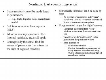
Nonlinear least squares regression

• Some models cannot be made linear in parameters
• E.g., theta-logistic stock-recruitment model
• Solution nonlinear least squares (NLS)
• All other assumptions from OLS (normal residuals,
  etc.) still apply
• Conceptually the same find the values of
  parameters that minimize the sum of squared
  residuals

• Numerically intensive cant be done by hand
• As number of parameters gets large say above
  10 or so can take substantial time even on
  modern computers
• Not guaranteed to get the right answer
• Computer algorithms find local minima
  sometimes there are more than one
• Need to provide pretty good initial guesses for
  the parameter values
• Base guesses on
• scientific information
• If only a few nonlinear parameters, try fixing
  them at a few values and using OLS to estimate
  the rest choose the best overall combination

2
NLS in R

• Need the nls library
• The function is nls()
• The formula is like a real equation, with all
  parameters specified
• Specify the initial values for the parameters
  (this also tells nls which things in the formula
  are parameters)
• Trace prints out the progress, which can be
  handy if things arent going well
• If the method doesnt converge, sometimes you can
  help things along by increasing maxiter or
  decreasing minFactor or tol

• library(nls)
• nls(
• log(Recruits) b0 b1log(Spawners)
  b2Spawnerstheta,
• startc(b0-11, b12.2, b2-3, theta.5),
• traceT,
• controlnls.control(maxiter100,
  minFactor1/2048, tol1e-4)
• )

3
Formula log(Recruits) b0 b1 log(Spawners)
b2 Spawnerstheta Parameters
Estimate Std. Error t value Pr(gtt) b0
28.5369 72.1780 0.395 0.695 b1
-2.0301 5.4898 -0.370 0.714 b2
-610.9205 4810.6300 -0.127 0.900 theta
-0.5404 1.4118 -0.383 0.704 Residual
standard error 0.7716 on 34 degrees of
freedom Correlation of Parameter Estimates
b0 b1 b2 b1 -0.9998
b2 0.9847 -0.9809 theta 0.9919
-0.9890 0.9988
4
(No Transcript)
5
(No Transcript)
6
Dangers of nonlinear regression

• You can get similarly good fits with very
  different looking functions
• OK for interpolating
• Different models will produce very different
  predictions when extrapolating

• For interpolating, we can find the best
  nonlinear model using nonparametric regression
• E.g., lowess (locally weighted sum of squares)
• This is what you see in diagnostic plots that try
  to indicate the nonlinear trend in residuals
  (e.g., CR plots)

7
(No Transcript)
8
(No Transcript)
9
Splines and GAM

• Another smoothing function is the cubic spline
• A bunch of cubic polynomials fit locally and
  joined together
• Allows us to fit a generalized additive model
  (GAM)

• Good when scientific theory tells us which
  variables should be important but not whether the
  effects should be nonlinear or what form of
  nonlinearity
• Can use GAM model directly for interpolation, or
  use to decide which nonlinear functions to use
  with nls

10
Family gaussian Link function identity
Formula Consumption s(Price) s(Income)
s(PNC/PUC) Parametric coefficients
Estimate std. err. t ratio
Pr(gtt) constant 385.05 0.4113
936.2 lt 2.22e-16 Approximate significance of
smooth terms edf chi.sq
p-value s(Price) 8.836 199.81
3.979e-06 s(Income) 6.889 280.43
2.4103e-07 s(PNC/PUC) 7.441 25.244
0.030148 R-sq.(adj) 0.998 Deviance explained
99.9 GCV score 18.525 Scale est. 6.0896
n 36
11
(No Transcript)
12
R code, part 1

• Attach the herring data
• fish lt- read.csv("Herring_BC.csv")
• attach(fish)
• Rerun the linear model to get initial parameter
  estimates
• fish.lm lt- lm(log(Recruits) log(Spawners)
  sqrt(Spawners))
• summary(fish.lm)
• Load the nls library, and take our first shot
  at the fit
• library(nls)
• fish.nls lt- nls(log(Recruits) b0
  b1log(Spawners) b2Spawnerstheta,
  startc(b0-11,b12.2,b2-.03,theta.5), traceT)
• Crank up the control parameters and try again
• fish.nls lt- nls(log(Recruits) b0
  b1log(Spawners) b2Spawnerstheta,
  startc(b0-11,b12.2,b2-.03,theta.5), traceT,
  controlnls.control(maxiter5000,minFactor1/16364
  0,tol1e-3))

13
R code, part 2

• Run a linear model to get starting values for a
  negative value of theta, and try again
• lm(log(Recruits) log(Spawners) I(1/Spawners))
• fish.nls lt- nls(log(Recruits) b0
  b1log(Spawners) b2Spawnerstheta,
  startc(b016,b1-1,b2-12000,theta-1), traceT,
  controlnls.control(maxiter5000,minFactor1/16364
  0,tol1e-3))
• summary(fish.nls)
• Look at some diagnostic plots of the residuals
• library(car)
• qq.plot(resid(fish.nls))
• plot(fitted(fish.nls),resid(fish.nls))
• abline(0,0,lty3)
• Plot the fitted values with the data
• plot(log(Spawners),log(Recruits))
• xx lt- seq(min(log(Spawners)),max(log(Spawners)),le
  ngth200)
• fish2.pred lt- predict(fish.nls,newdatadata.frame(
  Spawnersexp(xx)))
• lines(xx,fish2.pred)

14
R code, part 3

• Add the fitted values from the linear model
• fish1.pred lt- predict(fish.lm,newdatadata.frame(S
  pawnersexp(xx)))
• lines(xx,fish1.pred,lty2)
• Plot the data with a lowess regression
• plot(log(Spawners),log(Recruits))
• lines(lowess(log(Spawners),log(Recruits)))
• Load the gasoline data
• gas lt- read.csv("GasMarket2.csv")
• attach(gas)
• Fit a GAM
• library(modreg)
• gas.gam lt- gam(Consumption s(Price) s(Income)
  s(PNC/PUC))
• summary(gas.gam)
• plot(gas.gam)