Business and Economic Forecasting Chapter 5

1
Business and Economic ForecastingChapter 5

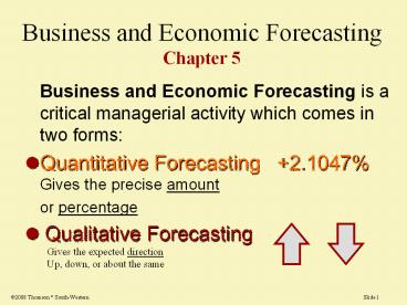
• Business and Economic Forecasting is a critical
  managerial activity which comes in two forms
• Quantitative Forecasting 2.1047 Gives the
  precise amount
• or percentage
• Qualitative Forecasting
• Gives the expected direction
• Up, down, or about the same

?2008 Thomson South-Western
2
Managerial ChallengeExcess Fiber Optic Capacity

• High-speed data installation grew exponentially
• But adoption follows a typical S-curve pattern,
  similar to the adoption rate of TV
• Access grew too fast, leading to excess capacity
  around the time of the tech bubble in 2001
• The challenge is to predict demand properly

100
Color TVs
Internet Access
1940 1960 1980 2000 2020
3
The Significance of Forecasting

• Both public and private enterprises operate under
  conditions of uncertainty.
• Management wishes to limit this uncertainty by
  predicting changes in cost, price, sales, and
  interest rates.
• Accurate forecasting can help develop strategies
  to promote profitable trends and to avoid
  unprofitable ones.
• A forecast is a prediction concerning the future.
  Good forecasting will reduce, but not eliminate,
  the uncertainty that all managers feel.

4
Hierarchy of Forecasts

• The selection of forecasting techniques depends
  in part on the level of economic aggregation
  involved.
• The hierarchy of forecasting is
• National Economy (GDP, interest rates, inflation,
  etc.)
• sectors of the economy (durable goods)
• industry forecasts (all automobile
  manufacturers)
• firm forecasts (Ford Motor Company)
• Product forecasts (The Ford Focus)

5
Forecasting Criteria

• The choice of a particular forecasting method
  depends on several criteria
• costs of the forecasting method compared with its
  gains
• complexity of the relationships among variables
• time period involved
• lead time between receiving information and the
  decision to be made
• accuracy needed in forecast

6
Accuracy of Forecasting

• The accuracy of a forecasting model is measured
  by how close the actual variable, Y, ends up to
  the forecasting variable, Y.
• Forecast error is the difference. (Y - Y)
• Models differ in accuracy, which is often based
  on the square root of the average squared
  forecast error over a series of N forecasts and
  actual figures
• Called a root mean square error, RMSE.
• RMSE ? ? (Y - Y)2 / N

7
Quantitative Forecasting

• Deterministic Time Series
• Looks For Patterns
• Ordered by Time
• No Underlying Structure
• Econometric Models
• Explains relationships
• Supply Demand
• Regression Models

Like technical security analysis
Like fundamental security analysis
8
Time SeriesExamine Patterns in the Past
Dependent Variable
X
X
X


Forecasted Amounts
TIME
To
The data may offer secular trends, cyclical
variations, seasonal variations, and random
fluctuations.
9
Time SeriesExamine Patterns in the Past
Dependent Variable
Secular Trend
X
X
X


Forecasted Amounts
TIME
To
The data may offer secular trends, cyclical
variations, seasonal variations, and random
fluctuations.
10
Time SeriesExamine Patterns in the Past
Dependent Variable
Secular Trend
Cyclical Variation
X
X
X


Forecasted Amounts
TIME
To
The data may offer secular trends, cyclical
variations, seasonal variations, and random
fluctuations.
11
Elementary Time Series Models for Economic
Forecasting
NO Trend

• Naive Forecast
• Yt1 Yt
• Method best when there is no trend, only random
  error
• Graphs of sales over time with and without trends
• When trending down, the Naïve predicts too high

?
?
?
?

?
?
time
Trend
?
?
?
?
?
time
12
2. Naïve forecast with adjustments for secular
trends

• Yt1 Yt (Yt - Yt-1 )
• This equation begins with last periods forecast,
  Yt.
• Plus an adjustment for the change in the amount
  between periods Yt and Yt-1.
• When the forecast is trending up, this adjustment
  works better than the pure naïve forecast method
  1.

13
3. Linear Trend 4. Constant rate of growth
Linear Trend Growth Uses a Semi-log
Regression

• Used when trend has a constant AMOUNT of change
• Yt a bT, where
• Yt are the actual observations and
• T is a numerical time variable

• Used when trend is a constant PERCENTAGE rate
• Log Yt a bT,
• where b is the continuously compounded growth
  rate

14
More on Constant Rate of Growth Modela proof

• Suppose Yt Y0( 1 G) t where g is the
  annual growth rate
• Take the natural log of both sides
• Ln Yt Ln Y0 t Ln (1 G)
• but Ln ( 1 G ) ? g, the equivalent continuously
  compounded growth rate
• SO Ln Yt Ln Y0 t g
• Ln Yt a b t
• where b is the growth rate

15
Numerical Examples 6 observations

• MTB gt Print c1-c3.
• Sales Time Ln-sales
• 100.0 1 4.60517
• 109.8 2 4.69866
• 121.6 3 4.80074
• 133.7 4 4.89560
• 146.2 5 4.98498
• 164.3 6 5.10169

Using this sales data, estimate sales in period
7 using a linear and a semi-log
functional form
16
The linear regression equation is Sales 85.0
12.7 Time Predictor Coef Stdev
t-ratio p Constant 84.987 2.417
35.16 0.000 Time 12.6514 0.6207
20.38 0.000 s 2.596 R-sq 99.0
R-sq(adj) 98.8
The semi-log regression equation is Ln-sales
4.50 0.0982 Time Predictor Coef
Stdev t-ratio p Constant 4.50416
0.00642 701.35 0.000 Time
0.098183 0.001649 59.54 0.000 s
0.006899 R-sq 99.9 R-sq(adj) 99.9
17
Forecasted Sales _at_ Time 7

• Linear Model
• Sales 85.0 12.7 Time
• Sales 85.0 12.7 ( 7)
• Sales 173.9

• Semi-Log Model
• Ln-sales 4.50 0.0982 Time
• Ln-sales 4.50 0.0982 ( 7 )
• Ln-sales 5.1874
• To anti-log
• e5.1874 179.0

linear
??
?
18

• Sales Time Ln-sales
• 100.0 1 4.60517
• 109.8 2 4.69866
• 121.6 3 4.80074
• 133.7 4 4.89560
• 146.2 5 4.98498
• 164.3 6 5.10169
• 179.0 7 semi-log
• 173.9 7 linear

Semi-log is exponential
7
Which prediction do you prefer?
19
5. Declining Rate of Growth Trend

• A number of marketing penetration models use a
  slight modification of the constant rate of
  growth model
• In this form, the inverse of time is used
• Ln Yt b1 b2 ( 1/t )
• This form is good for patterns like
  the one to the right
• It grows, but at continuously
  a declining rate

Y
time
20
6. Seasonal Adjustments The Ratio to Trend
Method

• Take ratios of the actual to the forecasted
  values for past years.
• Find the average ratio. This is the seasonal
  adjustment
• Adjust by this percentage by multiply your
  forecast by the seasonal adjustment
• If average ratio is 1.02, adjust forecast upward
  2

12 quarters of data
?
?
?
?
?
?
?
?
?
?
?
?
I II III IV I II III IV I II III IV
Quarters designated with roman numerals.
21
7. Seasonal Adjustments Dummy Variables

• Let D 1, if 4th quarter and 0 otherwise
• Run a new regression
• Yt a bT cD
• the c coefficient gives the amount of the
  adjustment for the fourth quarter. It is an
  Intercept Shifter.
• With 4 quarters, there can be as many as three
  dummy variables with 12 months, there can be as
  many as 11 dummy variables
• EXAMPLE Sales 300 10T 18D
• 12 Observations from the first quarter of 2005
  to 2007-IV.
• Forecast all of 2008.
• Sales(2008-I) 430 Sales(2008-II) 440
  Sales(2008-III) 450 Sales(2008-IV) 478

22
Soothing Techniques8. Moving Averages

• A smoothing forecast method for data that jumps
  around
• Best when there is no trend
• 3-Period Moving Ave is
• Yt1 Yt Yt-1 Yt-2/3
• For more periods, add them up and take the
  average

Dependent Variable



Forecast Line is Smoother


TIME
23
Smoothing Techniques9. First-Order Exponential
Smoothing

• A hybrid of the Naive and Moving Average methods
• Yt1 wYt (1-w)Yt
• A weighted average of past actual and past
  forecast, with a weight of w

• Each forecast is a function of all past
  observations
• Can show that forecast is based on geometrically
  declining weights.
• Yt1 w .Yt (1-w)wYt-1
• (1-w)2wYt-1
• Find lowest RMSE to pick the best w.

24
First-Order Exponential Smoothing Example for w
.50

• Actual Sales Forecast
• 100 100 initial seed required
• 120 .5(100) .5(100) 100
• 115
• 130
• ?

1 2 3 4 5
25
First-Order Exponential Smoothing Example for w
.50

• Actual Sales Forecast
• 100 100 initial seed required
• 120 .5(100) .5(100) 100
• 115 .5(120) .5(100) 110
• 130
• ?

1 2 3 4 5
26
First-Order Exponential Smoothing Example for w
.50

• Actual Sales Forecast
• 100 100 initial seed required
• 120 .5(100) .5(100) 100
• 115 .5(120) .5(100) 110
• 130 .5(115) .5(110) 112.50
• ? .5(130) .5(112.50) 121.25

1 2 3 4 5
Period 5 Forecast
MSE (120-100)2 (110-115)2 (130-112.5)2/3
243.75 RMSE ?243.75 15.61
27
Qualitative Forecasting10. Barometric
Techniques
Direction of sales can be indicated by other
variables.
Motor Control Sales
PEAK
peak
Index of Capital Goods
TIME
4 Months
Example Index of Capital Goods is a leading
indicator There are also lagging indicators and
coincident indicators
28
Time given in months from change

• LEADING INDICATORS
• M2 money supply (-14.4)
• SP 500 stock prices (-11.1)
• Building permits (-15.4)
• Initial unemployment claims (-12.9)
• Contracts and orders for plant and equipment
  (-7.3)

• COINCIDENT INDICATORS
• Nonagricultural payrolls (.8)
• Index of industrial production (-1.1)
• Personal income less transfer payment (-.4)
• LAGGING INDICATORS
• Prime rate (17.9)
• Change in labor cost per unit of output (6.4)

Survey of Current Business, 1995 See pages
182-183 in the textbook
29
Handling Multiple Indicators

• Diffusion Index Suppose 11 forecasters predict
  stock prices in 6 months, up or down. If 4
  predict down and seven predict up, the Diffusion
  Index is 7/11, or 63.3.
• above 50 is a positive diffusion index
• Composite Index One indicator rises 4 and
  another rises 6. Therefore, the Composite Index
  is a 5 increase.
• used for quantitative forecasting

30
Qualitative Forecasting11. Surveys and Opinion
Polling Techniques
Common Survey Problems

• Sample bias--
• telephone, magazine
• Biased questions--
• advocacy surveys
• Ambiguous questions
• Respondents may lie on questionnaires

New Products have no historical data --
Surveys can assess interest in new ideas.
Survey Research Center of U. of Mich. does
repeat surveys of households on Big Ticket items
(Autos)
31
Qualitative Forecasting12. Expert Opinion

• The average forecast from several experts is a
  Consensus Forecast.
• Mean
• Median
• Mode
• Truncated Mean
• Proportion positive or negative

32

• EXAMPLES
• IBES, First Call, and Zacks Investment --
  earnings forecasts of stock analysts of companies
• Conference Board macroeconomic predictions
• Livingston Surveys--macroeconomic forecasts of
  50-60 economists
• Individual economists tend to be less accurate
  over time than the consensus forecast.

33
13. Econometric Models

• Specify the variables in the model
• Estimate the parameters
• single equation or perhaps several stage methods
• Qd a bP cI dPs ePc
• But forecasts require estimates for future
  prices, future income, etc.
• Often combine econometric models with time series
  estimates of the independent variable.
• Garbage in Garbage out

34
example

• Qd 400 - .5P 2Y .2Ps
• anticipate pricing the good at P 20
• Income (Y) is growing over time, the estimate is
  Ln Yt 2.4 .03T, and next period is T 17.
• Y e2.910 18.357
• The prices of substitutes are likely to be P
  18.
• Find Qd by substituting in predictions for P, Y,
  and Ps
• Hence Qd 430.31

35
14. Stochastic Time Series

• A little more advanced methods incorporate into
  time series the fact that economic data tends to
  drift
• yt a byt-1 et
• In this series, if a is zero and b is 1, this is
  essentially the naïve model. When a is zero, the
  pattern is called a random walk.
• When a is positive, the data drift. The
  Durbin-Watson statistic will generally show the
  presence of autocorrelation, or AR(1), integrated
  of order one.
• One solution to variables that drift, is to use
  first differences.

36
Cointegrated Time Series

• Some econometric work includes several stochastic
  variable, each which exhibits random walk with
  drift
• Suppose price data (P) has positive drift
• Suppose GDP data (Y) has positive drift
• Suppose the sales is a function of P Y
• Salest a bPt cYt
• It is likely that P and Y are cointegrated in
  that they exhibit comovement with one another.
  They are not independent.
• The simplest solution is to change the form into
  first differences as in DSalest a bDPt
  cDYt