More QSAR

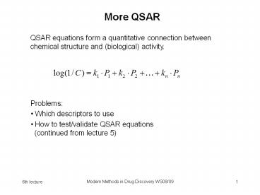
1
More QSAR
QSAR equations form a quantitative connection
between chemical structure and (biological)
activity.

• Problems
• Which descriptors to use
• How to test/validate QSAR equations (continued
  from lecture 5)

2
Evaluating QSAR equations (III)
(Simple) k-fold cross validation Partition your
data set that consists of N data points into k
subsets (k lt N).
k times
Generate k QSAR equations using a subset as test
set and the remaining k-1 subsets as training set
respectively. This gives you an average error
from the k QSAR equations.
In practice k 10 has shown to be reasonable(
10-fold cross validation)
3
Evaluating QSAR equations (IV)
Leave one out cross validation Partition your
data set that consists of N data points into k
subsets (k N).
N times

• Disadvantages
• Computationally expensive
• Partitioning into training and test set is more
  or less by random, thus the resulting average
  error can be way off in extreme cases.

Solution (feature) distribution within the
training and test sets should be identical or
similar
4
Evaluating QSAR equations (V)
Stratified cross validation Same as k-fold cross
validation but each of the k subsets has a
similar (feature) distribution.
k times
The resulting average error is thus more prone
against errors due to inequal distribution
between training and test sets.
5
Evaluating QSAR equations (VI)
alternativeCross-validation and leave one out
(LOO) schemes
Leaving out one or more descriptors from the
derived equation results in the cross-validated
correlation coefficient q2. This value is of
course lower than the original r2. q2 being much
lower than r2 indicates problems...
6
Evaluating QSAR equations (VII)
Problems associated with q2 and leave one out
(LOO) ? There is no correlation between q2 and
test set predictivity, q2 is related to r2 of the
training set
Kubinyis paradoxon Most r2 of test sets are
higher than q2 of the corresponding training sets
Lit A.M.Doweyko J.Comput.-Aided Mol.Des. 22
(2008) 81-89.
7
Evaluating QSAR equations (VIII)
One of most reliable ways to test the performance
of a QSAR equation is to apply an external test
set.? partition your complete set of data into
training set (2/3) and test set (1/3 of all
compounds, idealy) compounds of the test set
should be representative(confers to a 1-fold
stratified cross validation)? Cluster analysis
8
Interpretation of QSAR equations (I)

• The kind of applied variables/descriptors should
  enable us to
• draw conclusions about the underlying
  physico-chemical processes
• derive guidelines for the design of new
  molecules by interpolation

Higher affinity requires more fluorine, less OH
groups

• Some descriptors give information about the
  biologicalmode of action
• A dependence of (log P)2 indicates a transport
  process of the drug to its receptor.
• Dependence from ELUMO or EHOMO indicates a
  chemical reaction

9
Correlation of descriptors
Other approaches to handle correlated descriptors
and/or a wealth of descriptors

• Transforming descriptors to uncorrelated
  variables by
• principal component analysis (PCA)
• partial least square (PLS)
• comparative molecular field analysis
  (CoMFA)Methods that intrinsically handle
  correlated variables
• neural networks

10
Partial least square (I)
The idea is to construct a small set of latent
variables ti (that are orthogonal to each other
and therefore uncorrelated) from the pool of
inter-correlated descriptors xi .
In this case t1 and t2 result as the normal modes
of x1 and x2 where t1 shows the larger variance.
11
Partial least square (II)
The predicted term y is then a QSAR equation
using the latent variables ti
where
The number of latent variables ti is chosen to be
(much) smaller than that of the original
descriptors xi. But, how many latent variables
are reasonable ?
12
Principal Component Analysis PCA (I)
Problem Which are the (decisive) significant
descriptors ?
Principal component analysis determines the
normal modes from a set of descriptors/variables.
This is achieved by a coordinate transformation
resulting in new axes. The first principal
component then shows the largest variance of the
data. The second and further normal components
are orthogonal to each other.
13
Principal Component Analysis PCA (II)
The first component (pc1) shows the largest
variance, the second component the second largest
variance, and so on.
Lit E.C. Pielou The Interpretation of
Ecological Data, Wiley, New York, 1984
14
Principal Component Analysis PCA (III)
The significant principal components usually have
an eigen value gt1 (Kaiser-Guttman criterium).
Frequently there is also a kink that separates
the less relevant components (Scree test)
15
Principal Component Analysis PCA (IV)
The obtained principal components should account
for more than 80 of the total variance.
16
Principal Component Analysis (V)
Example What descriptors determine the logP ?
property pc1 pc2 pc3 dipole moment
0.353 polarizability 0.504 mean of ESP
0.397 -0.175 0.151 mean of ESP -0.389 0.104
0.160 variance of ESP 0.403 -0.244 minimum
ESP -0.239 -0.149 0.548 maximum ESP 0.422
0.170 molecular volume 0.506 0.106 surface
0.519 0.115 fraction of totalvariance 28
22 10
Lit T.Clark et al. J.Mol.Model. 3 (1997) 142
17
Comparative Molecular Field Analysis (I)
The molecules are placed into a 3D grid and at
each grid point the steric and electronic
interaction with a probe atom is calculated
(force field parameters)
For this purpose the GRID program can be
used P.J. GoodfordJ.Med.Chem. 28 (1985) 849.
Problems active conformation of the molecules
needed All molecule must be superimposed (aligned
according to their similarity)
Lit R.D. Cramer et al. J.Am.Chem.Soc. 110 (1988)
5959.
18
Comparative Molecular Field Analysis (II)
The resulting coefficients for the matrix S (N
grid points, P probe atoms) have to determined
using a PLS analysis.
19
Comparative Molecular Field Analysis (III)
Application of CoMFAAffinity of steroids to the
testosterone binding globulin
Lit R.D. Cramer et al. J.Am.Chem.Soc.110 (1988)
5959.
20
Comparative Molecular Field Analysis (IV)
Analog to QSAR descriptors, the CoMFA variables
can be interpreted. Here (color coded) contour
maps are helpful
yellow regions of unfavorable steric
interactionblue regions of favorable steric
interaction
Lit R.D. Cramer et al. J.Am.Chem.Soc. 110 (1988)
5959
21
Comparative Molecular Similarity Indices
Analysis (CoMSIA)
CoMFA based on similarity indices at the grid
points
Comparison of CoMFA and CoMSIA potentials shown
along one axis of benzoic acid
Lit G.Klebe et al. J.Med.Chem. 37 (1994) 4130.
22
Neural Networks (I)
Neural networks can be regarded as a common
implementation of artificial intelligence. The
name is derived from the network-like connection
between the switches (neurons) within the system.
Thus they can also handle inter-correlated
descriptors.
modeling of a (regression) function
From the many types of neural networks,
backpropagation and unsupervised maps are the
most frequently used.
23
Neural Networks (II)
A typical backpropagation net consists of neurons
organized as the input layer, one or more hidden
layers, and the output layer
Furthermore, the actual kind of signal
transduction between the neurons can be different
24
Recursive Partitioning

• Instead of quantitative values often there is
  only qualitative information available, e.g.
  substrates versus non-substrates
• Thus we need classification methods such as
• decision trees
• support vector machines
• (neural networks) partition at what score value
  ?

Picture J. Sadowski H. Kubinyi J.Med.Chem. 41
(1998) 3325.
25
Decision Trees
Iterative classification
Advantages Interpretation ofresults, design of
newcompoundswithdesiredproperties Disadvantag
eLocal minima problemchosing the descriptors
ateach branching point
Lit J.R. Quinlan Machine Learning 1 (1986) 81.
26
Support Vector Machines
Support vector machines generate a hyperplane in
the multi-dimensional space of the descriptors
that separates the data points.
Advantages accuracy, a minimum of descriptors(
support vectors) used Disadvantage
Interpretation of results, design of new
compounds with desired properties, which
descriptors for input
27
Property prediction So what ?
Classical QSAR equations small data sets, few
descriptors that are (hopefully) easy to
understand
CoMFA small data sets, many
descriptors
Partial least square small data sets,
many descriptors
interpretation of results often difficult
Neural nets large data sets,
some descriptors
black box methods
Support vector machines large data sets,
many descriptors
28
Interpretation of QSAR equations (II)
Caution is required when extrapolating beyond the
underlying data range. Outside this range no
reliable predicitions can be made
Beyond theblack stump ...
Kimberley, Western Australia
29
Interpretation of QSAR equations (III)
There should be a reasonable connection between
the used descriptors and the predicted
quantity. Example H. Sies Nature 332 (1988)
495. Scientific proof that babies are delivered
by storks
According data can be found at /home/stud/mihu004/
qsar/storks.spc
30
Interpretation of QSAR equations (IV)
Another striking correlation QSAR has evolved
into a perfectly practiced art of logical fallacy
S.R. Johnson J.Chem.Inf.Model. 48 (2008) 25.
? the more descriptors are available, the higher
is the chance of finding some that show a chance
correlation
31
Interpretation of QSAR equations (V)
Predictivity of QSAR equations in between data
points. The hypersurface is not smooth activity
islands vs. activity cliffs
Bryce Canyon National Park, Utah
Lit G.M. Maggiora J.Chem.Inf.Model. 46 (2006)
1535.
S.R. Johnson J.Chem.Inf.Model. 48 (2008) 25.
32
Interpretation of QSAR equations (VI)

• What QSAR performance is realistic?
• standard deviation (se) of 0.20.3 log units
  corresponds to a typical 2-fold error in
  experiments (soft data). This gives rise to an
  upper limit of
• r2 between 0.770.88 (for biological systems)
• ? obtained correlations above 0.90 are highly
  likely to be accidental or due to overfitting
  (except for physico-chemical properties that
  show small errors, e.g. boiling points, logP,
  NMR 13C shifts)But even random correlations
  can sometimes beas high as 0.84

Lit A.M.Doweyko J.Comput.-Aided Mol.Des. 22
(2008) 81-89.
33
Interpretation of QSAR equations (VII)
According to statistics more people die after
being hit by a donkey than from the consequences
of an airplane crash.