STT 430/530, Nonparametric Statistics - PowerPoint PPT Presentation
1 / 7
Title:
STT 430/530, Nonparametric Statistics
Description:
3 pivot quantities on which to base bootstrap ... D.V (1997) Bootstrap Methods and Their Applications and Lunneborg ... Nonparametric Statistics Author: Dargan ... – PowerPoint PPT presentation
Number of Views:17
Avg rating:3.0/5.0
Title: STT 430/530, Nonparametric Statistics
1
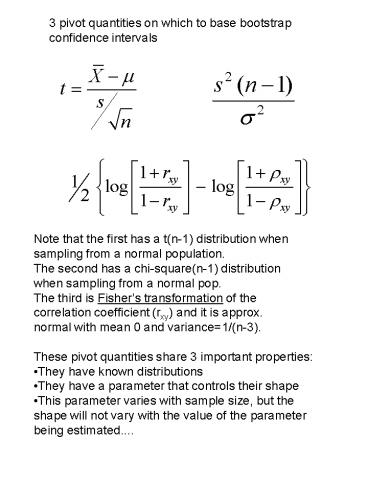
3 pivot quantities on which to base bootstrap
confidence intervals
- Note that the first has a t(n-1) distribution
when - sampling from a normal population.
- The second has a chi-square(n-1) distribution
- when sampling from a normal pop.
- The third is Fishers transformation of the
- correlation coefficient (rxy) and it is approx.
- normal with mean 0 and variance1/(n-3).
- These pivot quantities share 3 important
properties - They have known distributions
- They have a parameter that controls their shape
- This parameter varies with sample size, but the
- shape will not vary with the value of the
parameter - being estimated....
2
- As the Students t distribution takes away the
mean and divides by the s.e. of the sample mean,
so we codify this process and call it
Studentization for any estimator t of q . - Well use the bootstrap form of the Studentized
estimate to construct various bootstrap
confidence intervals...
3
- So heres the way to do this for the mean.
- compute the sample mean and sample s.d. from
the original data - obtain a bootstrap sample of size n from the
original data and compute the bootstrap mean,
and the bootstrap standard - deviation, sb.
- now compute the bootstrap t-pivot quantity
- now repeat this step at least 1000 times to get
the bootstrap distribution of tb . - let tb, .025 and tb, .975 be the .025 and
.975 quantiles of the bootstrap distribution of
tb . Construct the 95 confidence interval for m
as - Now implement this in R... try with the latch
failure data in Table 1.2.1
4
- Bootstrap confidence intervals for the population
standard deviation, s, can be done with the
c2-pivot - If the sample is from a normal distribution, then
the c2-pivot has a chi-square distribution with
n-1 degrees of freedom and a 95 confidence
interval for sigma can be computed as - If normality is not a reasonable assumption, then
well use the bootstrap as follows - compute the sample variance s2 for the original
sample data. - bootstrap the sample of size n and compute the
bootstrap sample variance and the bootstrap
c2-pivot quantity - (here, sb2 is the bootstrap sample variance)
- now repeat 1000 times or more to get the
bootstrap distribution of the bootstrapped
c2-pivots
5
- then the bootstrap 95 CI for the population
variance is - take the square root if you want confidence
intervals for sigma... - Implement this in R... again on the Table 1.2.1
data. - Here are the problems from the textbook that are
due at the final exam time. Be sure to write up
the solution so I can tell that you understand
the methods and the context of the problem.
Include appropriate R output to illustrate your
solutions... - p.106 6
- p.141ff 4,5,6 (second part), 7,9
- p.189ff 1,3,4,5,7,8,9(a),12,13
- p.298ff 1,5,7
- On the last class day I will give you some data
that will form the basis for the final exam the
next week. - See page 258 for a chart of Coverage Percentages
in a simulation done by the author for various
underlying distributions - make sure you
understand the conclusions of that discussion
6
- See section 8.3 for a discussion of three
additional methods for computing bootstrap
confidence intervals in more generality The
three methods are - Percentile method
- Residual method
- BCA method (BCAbias corrected and accelerated)
- Suppose we are trying to estimate the unknown
population parameter ? - use based on a
sample of size n from the population. - The percentile method constructs the CI by
bootstrapping the estimator to get its
distribution - in particular its .025 and .975
quantiles. Construct the 95 CI for ? as - The residual method estimates ? by first getting
the bootstrap distribution of the residuals - and then constructing the 95 CI for ? as
7
- The BCA method is more complex and a discussion
of it is given in section 8.3.2. If youre
interested in pursuing this method look at the R
package called boot . More details can be found
in Davison, A.C. and Hinkley, D.V (1997)
Bootstrap Methods and Their Applications and
Lunneborg, C.E. (2000) Data Analysis by
Resampling Concepts and Applications.


