
Multiple Linear Regression - Matrix Formulation - PowerPoint PPT Presentation
Title:
Multiple Linear Regression - Matrix Formulation
Description:
Notice command for matrix multiplication. The inverse of X'X can also be obtained. by using R ... t tables using 4 degrees of freedom give cut of point of 2. ... – PowerPoint PPT presentation
Number of Views:437
Avg rating:3.0/5.0
Title: Multiple Linear Regression - Matrix Formulation
1
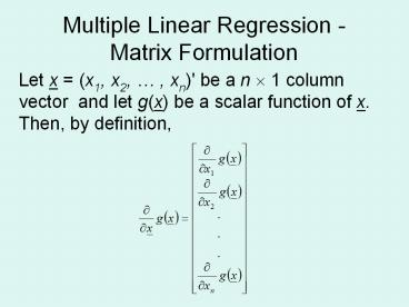
Multiple Linear Regression - Matrix Formulation
Let x (x1, x2, , xn)' be a n ? 1 column
vector and let g(x) be a scalar function of x.
Then, by definition,
2
For example, let
Let a (a1, a2, , a n)' be a n ? 1 column
vector of constants. It is easy to verify that
and that, for symmetrical A (n ? n)
3
Theory of Multiple Regression
Suppose we have response variables Yi , i 1,
2, , n and k explanatory variables/predictors
X1, X2, , Xk .
i 1,2, , n There are k2 parameters b0 , b1
, b2 , , bk and s2
4
X is called the design matrix
5
6
OLS (ordinary least-squares) estimation
7
(No Transcript)
8
Fitted values are given by
H is called the hat matrix ( it puts the
hats on the Ys)
9
The error sum of squares, SSRES , is
The estimate of s2 is based on this.
10
Example Find a model of the form
for the data below.
y x1 x2
3.5 3.1 30
3.2 3.4 25
3.0 3.0 20
2.9 3.2 30
4.0 3.9 40
2.5 2.8 25
2.3 2.2 30
11
X is called the design matrix
12
The model in matrix form is given by
We have already seen that
Now calculate this for our example
13
R can be used to calculate XX and the answer is
14
To input the matrix in R use Xmatrix(c(1,1,1,1,
1,1,1,3.1,3.4,3.0,3.4, 3.9,2.8,2.2,30,25,20,30,40,
25,30),7,3)
Number of rows
Number of columns
15
(No Transcript)
16
(No Transcript)
17
Notice command for matrix multiplication
18
The inverse of XX can also be obtained by using
R
19
We also need to calculate XY
Now
20
Notice that this is the same result as obtained
previously using the lm result on R
21
So y -0.2138 0.8984x1 0.01745x2 e
22
The hat matrix is given by
23
The fitted Y values are obtained by
24
Recall once more we are looking at the model
25
Compare with
26
Error Terms and Inference
A useful result is
n number of points k number of explanatory
variables
27
In addition we can show that
where s.e.(bi)?c(i1)(i1)?
And c(i1)(i1) is the (i1)th diagonal element
of
28
For our example
29
was calculated as
30
This means that c11 6.683, c220.7600,c330.0053
Note that c11 is associated with b0, c22 with b1
and c33 with b2
We will calculate the standard error for b1 This
is ?0.7600 x 0.2902 0.2530
31
The value of b1 is 0.8984 Now carry out a
hypothesis test. H0 b1 0 H1 b1 ? 0 The
standard error of b1 is 0.2530
32
The test statistic is This calculates as
(0.8984 0)/0.2530 3.55
33
Ds.. .
................
t tables using 4 degrees of freedom give cut of
point of 2.776 for 2.5.
34
We therefore accept H1. There is no evidence at
the 5 level that b1 is zero. The process can be
repeated for the other b values and confidence
intervals calculated in the usual way.
CI for ?2 - based on the ?42 distribution of
((4 ? 0.08422)/11.14 , (4 ? 0.08422)/0.4844)
i.e. (0.030 , 0.695)
35
The sum of squares of the residuals can also be
calculated.