
Fluid Simulation A Practical Approach: Part I - PowerPoint PPT Presentation
1 / 32
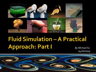
Title:
Fluid Simulation A Practical Approach: Part I
Description:
Broad view of the fluid simulation in graphics community and its ... Movie special effects (Finding Nemo, Pirates of Caribbean) Medical simulation (Blood flow) ... – PowerPoint PPT presentation
Number of Views:549
Avg rating:3.0/5.0
Title: Fluid Simulation A Practical Approach: Part I
1
Fluid Simulation A Practical Approach Part I
- By Michael Su
04/16/2009
2
Agenda
- Introduction
- Fluid characteristics
- Navier-Stokes equation
- Eulerian vs. Lagrangian approach
- Dive into the glory detail (A case study of the
2d fluid simulation) - Advection
- Diffusion
- Pressure solve
- Fluid object couple
- One-way and two-way coupling
- Real-time fluids
3
Objectives
- Broad view of the fluid simulation in graphics
community and its potential applications - Basic knowledge about the grid-based fluid
simulation - Understanding the challenges of the existing
methods - Foundation for the following two fluids- related
lectures (smoke granular material).
4
Introduction
- Applications
- Games (Half Life, Crysis)
- Scientific visualization (Water sewage system,
dam construction) - Movie special effects (Finding Nemo, Pirates of
Caribbean) - Medical simulation (Blood flow)
- What can we achieve so far?
- Smoke
- Granular flow (Sand)
- Newtonian fluid (Water, ocean)
- Non-Newtonian fluid (Blood, honey, goop
(viscoelaticity flow)) - Microscopic phenomena
5
Fluid Characteristics (1)
- Basic properties
- Pressure
- Density
- Viscosity (subject to shear stress)
- Surface tension
- Different types of fluids
- Incompressible (divergence-free) fluids Fluids
doesnt change volume (very much). - Compressible fluids Fluids change their
- volume significantly.
- Viscous fluids Fluids tend to resist a
- certain degrees of deformation
6
Fluid Characteristics (2)
- Inviscid (Ideal) fluids Fluids dont have
resistance to the shear stress - Turbulent flow Flow that appears to have chaotic
and random changes - Laminar (streamline) flow Flow that has
- smooth behavior
- Newtonian fluids Fluids continue
- to flow, regardless of the force
- acting on it
7
Fluid Characteristics (3)
- Non-Newtonian fluids Fluids that have
non-constant viscosity - Phase Transition Fluids may change
- physical behavior under different
- environmental conditions.
8
Challenges
- Modeling continuum fluids on discrete systems
Its all about approximations - Topological variations and different kinds of
behaviors with interacting subjects - Numerical stabilities, accuracy and convergence
issues - Performance
- User control
9
Fluid Simulation A Practical Approach Part II
- By Michael Su
04/20/2009
10
Calculus Review (1)
- Gradient ( ) A vector pointing
- in the direction of the greatest
- rate of increment
- Divergence ( ) Measure how the
- vectors are converging or diverging
- at a given location (volume
- density of the outward flux)
u can be a scalar or a vector
Source, Div(u) 0
Sink, Div(u)
u can only be a vector
11
Calculus Review (2)
- Laplacian (? or ) Divergence of the
gradient - Finite Difference Derivative approximation
u can be a scalar or a vector
12
Navier-Stokes Equation
- Momentum equation
- Incompressibility
ut k?2u (u??)u ?p f
George Gabriel Stokes (18191903)
Claude-Louis Navier (17851836)
??u0
u the velocity field
k kinematic viscosity
13
Techniques Overview
- Borrowed from CFD (Computational Fluid Dynamics)
- Common techniques for solving Navier Stokes
equation - Eulerian approach (grid-based)
- Lagrangian approach (particle-based)
- Spectral method
- Lattice Boltzmann method
14
Eulerian Approach
- Discretize the domain using finite differences
- Define scalar vector fields on the grid
- Use the operator splitting
- technique to solve each
- term separately
- Evaluation
- Derivative approximation
- Adaptive time step/solver
- Memory usage speed
- Grid artifact/resolution limitation
15
Lagrangian Approach
- Treat the fluid as discrete particles
- Apply interaction forces (i.e. pressure/viscosity)
according to certain - pre-defined smoothing kernels
- Evaluations
- Mass / Momentum conservation
- More intuitive
- Fast, no linear system solving
- Connectivity information/Surface reconstruction
16
Case Study A 2D Fluid Simulator
- We focus exclusively on incompressible, viscous
fluid - Assuming the gravity is the only external force
- No inflow or outflow
- Constant viscosity, constant density everywhere
in the fluid
17
Simulation Loop
Advection
Body Force
Diffusion
Scalar/Vector fields defined on the grid
Pressure Solve
ut k?2u (u??)u ?p f
??u0
18
The Power of Operator Splitting
- One complicated Multi-dimensional operator A
series of simple, lower dimensional operators - Each operator can have its own integration scheme
and different time step sizes - High modularity and easy to debug
Un A B D P
U
U
U
Un1
19
Advection (1)
- Sometimes called Convection or Transport
- Define how a quantity moves with the underlying
velocity field - This term ensures the conservation of momentum
- Advection equation
- Approaches
- Forward Euler (unstable)
- Semi-Lagragian advection (stable for large time
steps, but suffers from the dissipation issue)
20
Advection (2)
Forward Euler Advection
Semi-Lagragian Advection
21
Diffusion (1)
- Define how a quantity in a cell inter-changes
with its neighbors - Diffusion Blurring
- The viscous fluid can be achieved by applying
diffusion to the velocity field
Low Viscosity
High Viscosity
Figures from Carlson, Mucha, Turk Melting and
Flowing, SCA 02
22
Diffusion (2)
- Diffusion equation
- Approaches
- Explicit formulation
- Implicit formulation
- (for high viscosity)
23
Diffusion (3)
0
0
0
0
2.5
5
0
0
0
0
-10
2.5
2.5
0
0
0
0
0
0
2.5
0
Before the diffusion
After the diffusion (k 0.5, time step size 1)
24
Pressure Solve (1)
- Its sometimes called Pressure Projection
- What does the pressure do?
- Keep the fluid at constant volume
(incompressible, conservation of mass). - Make sure the velocity field stays
divergence-free
Compressible
Incompressible
25
Pressure Solve (2)
- Equation to solve
- How to solve for pressure
- Taking divergence of both sides of (1), we will
have - Build a system of equations and solve Ap d
using an iterative method such as Conjugate
Gradient - Update the velocity field from the pressure
gradient
s.t.
(1)
(Poisson Equation)
26
Pressure Solve (3)
- What about the pressure on boundary nodes?
- Free surface The fluid can
- evolve freely (p 0)
- Solid wall The fluid cant
- penetrate the wall but can
- flow freely in tangential
- directions (Neumann BC)
27
Issues
- Possible reasons why your simulation doesnt look
right - CFL condition violation
- Smaller time steps / Implicit solver
- Flux conservation BCs may not be set correctly
- Grid resolution/ Memory Adaptive grids
- Numerical dissipation Back and Forth Error
Compensation and Correction 4 / Vorticity
confinement 5 - Handle the interface and complex topological
changes Level set method 6 - Volume loss Particle level set 7
28
Fluid-Object Coupling
- One-way coupling
- Solid-Fluid interaction The fluid has no
influence on the solid - Fluid-Solid interaction The solid has no
influence on the fluid - Two-way coupling
- Manipulate the boundary conditions
- Finite Element techniques ALE DLM
- Rigid Fluid Treat the solid as fluids and
enforce the rigidity constraint 8
29
Real-time Fluids (1)
- Principles
- Cheap to compute
- Low memory consumption
- Stability
- Plausibility
- Interactivity
- Common techniques
- Procedural water Superimpose sine waves of a
variety of amplitudes and directions. 9
30
Real-time Fluids (2)
- Heightfield approximations If the surface is the
only interest, it can be represented using a 2d
heightfield and animated by 2d wave equations
with interaction forces. - Particle systems This approach is
- good at simulating a small amount of
- water such as a puddle, a bubble,
- or splashing fluids
31
References (1)
- 1 R. Bridson and M. Müller-Fischer. Fluid
Simulation. SIGGRAPH 07 Course Notes - 2 R. Bridson. Fluid Simulation for Computer
Graphics. A K Peters, 2008 - 3 J. Stam. Real-Time Fluid Dynamics for Games.
GDC 2003 - 4 B. Kim, Y. Liu, I. Llamas, and J. Rossignac.
FlowFixer Using BFECC for Fluid Simulation.
EGWNP 05 - 5 R. Fedkiw, J. Stam, and H.W. Jenson. Visual
Simulation of Smoke. SIGGRAPH 01 - 6 N. Foster, R. Fedkiw, Practical Animation of
Liquids. SIGGRAPH 01 - 7 D. Enright, S. Marschner, R. Fedkiw.
Animation and Rendering of Complex Water
Surfaces. SIGGRAPH 02 - 8 M. Carlson, P. J. Mucha, G. Turk. Rigid
Fluid Animating the Interplay Between Rigid
Bodies and Fluid. SIGGRAPH 04
32
References (2)
- 9 D. Hinsinger, F. Neyret, M. Cani. Interactive
Animation of Ocean Waves. SCA 02
Recommended
CrystalGraphics Presentations


