1' INTRODUCTION GENERAL PRINCIPLES AND BASIC CONCEPTS

1

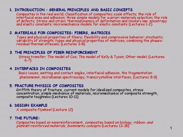
• 1. INTRODUCTION GENERAL PRINCIPLES AND BASIC
  CONCEPTS
• Composites in the real world Classification of
  composites scale effects the role of
  interfacial area and adhesion three simple
  models for a-priori materials selection the role
  of defects Stress and strain thermodynamics of
  deformation and Hookes law anisotropy and
  elastic constants micromechanics models for
  elastic constants Lectures 1-2
• 2. MATERIALS FOR COMPOSITES FIBERS, MATRICES
• Types and physical properties of fibers
  flexibility and compressive behavior stochastic
  variability of strength types and physical
  properties of matrices combining the phases
  residual thermal stresses Lectures 3-5
• 3. THE PRINCIPLES OF FIBER REINFORCEMENT
• Stress transfer The model of Cox The model of
  Kelly Tyson Other model Lectures 6-7
• 4. INTERFACES IN COMPOSITES
• Basic issues, wetting and contact angles,
  interfacial adhesion, the fragmentation
• phenomenon, microRaman spectroscopy,
  transcrystalline interfaces, Lectures 8-9
• 5. FRACTURE PHYSICS OF COMPOSITES
• Griffith theory of fracture, current models for
  idealized composites, stress concentration,
  simple mechanics of materials, micromechanics of
  composite strength, composite toughness Lectures
  10-11
• 6. DESIGN EXAMPLE
• A composite flywheel Lecture 12

2

• FRACTURE PHYSICS OF COMPOSITES
• Material Strength Griffiths early approach
• Homogeneous and isotropic solid
• Goal to calculate the strength of the solid and
  compare with experimental results.
• The application of a stress causes an increase in
  the energy of the system.
• Around the equilibrium point (the minimum of the
  potential energy), the stress varies linearly
  with distance ( Hookes behavior).
• However, for larger distances, the stress reaches
  a maximum at the point of inflection of the
  energy-separation curve.

3
smax
a0
l/2
4
Orowan (1949 Polanyi (1921)

• Theoretical strength is seen to increase if
  interatomic spacing decreases, and if Youngs
  modulus and fracture energy increase. Thus, when
  looking for strong solids, atoms with small ionic
  cores are preferred Beryllium, Boron, Carbon,
  Nitrogen, Oxygen, Aluminum, Silicon etc - the
  strongest materials always contain one of these
  elements.
• Using the O-P expression above, it is found that
  the theoretical strength can be approximated by
  (for most solids)

In practice, the tensile strength is much less
than E/10 because of the omnipresence of defects.
5
Example a hole in a plate (Inglis, 1913)
(b)
Note Purely geometric effect!
6
(No Transcript)
7
Griffiths theory

• Brittle solids contain defects
• Griffiths original query
• What is the strength of a brittle solid if a
  realistic, sharp crack of length a is present?
• Alternatively At which applied stress will a
  crack of length a start to propagate?
• Remember the prediction

This gave too high a prediction because no defects
8
Griffiths Assumptions Sharp crack in infinite,
thin plate (thickness t) Self-similar crack
propagation
Solution A balance must be struck between the
decrease in potential energy and the increase in
surface energy resulting from the presence of a
crack. (The surface energy arises from the fact
that there is a non-equilibrium configuration of
nearest neighbor atoms at any surface in a
solid).
9
Basic idea around the crack 2a, a volume
approximately equal to a circular cylinder
carries no stress and thus there is a reduction
in strain energy
s

2a
s
In fact, Griffith showed that the actual strain
energy reduction is
10
There exists an energy balance between (1) strain
energy decrease as the crack extends (negative),
and (2) surface energy increase necessary for the
formation of the new crack surfaces
The total energy balance is thus
The following plot shows the roles of the
conflicting energetic contributions
11
Plot of total energy UT against crack length
Below the critical crack length, the crack is
stable and does not spontaneously grow. Beyond
the critical crack length (at equilibrium), the
crack propagates spontaneously without limit.
12
The condition for spontaneous propagation is
(Griffith, 1921)
This is a (thermodynamics-based) necessary
condition for fracture in solids. Note the math
is similar to nucleation in phase transition Note
that if the Orowan-Polanyi expression
is combined with Inglis expression for an
ellipse
13
We obtain
Griffith
Correction factor
The correction factor amounts to about 0.6 if r
a0, and to about 0.8 if r 2a0. This gives
confidence in the result.
In 1930, Obreimoff carried out an experiment on
the cleavage of mica, using a different
experimental configuration. Contrasting with the
Griffith experiment, the equilibrium
configuration used by Obreimoff proves to be
stable
14
(No Transcript)
15
Griffiths model clearly demonstrates that large
cracks or defects lower the strength of a material

• But then, what is the physical meaning of the
  strength
• of a material?? Is this parameter meaningful at
  all?
• The strength is not a material constant !
• Deeper insight is necessary to quantify fracture
  in a more universal way
• This leads to the field of Linear Elastic
  Fracture Mechanics (or LEFM), developed in the
  1950s by Irwin and others

16
FIRST WAY OF REWRITING GRIFFITHS EQUATION
Two variables s and a
Only material properties This is a constant
Fracture criterion Fracture occurs when the
left-hand side product reaches the critical value
given in the right-hand side expression, which is
a new material constant with non-intuitive units
(MPa m1/2)
17
The Stress intensity factor (a variable)
The fracture toughness (a constant)
Fracture occurs when K becomes equal to Kc
18
SECOND WAY OF REWRITING GRIFFITHS EQUATION
Two variables s and a
Only material property This is a constant
Fracture criterion Fracture occurs when the
left-hand side product reaches the critical value
given in the right-hand side expression, which is
a new material constant with energy units
19
The energy release rate Or Crack driving force (a
variable)
The materials resistance to crack extension (a
constant)
Fracture occurs when G becomes equal to Gc
20
Fracture of Composites(An introduction)

• Is LEFM applicable to composites?
• Assumption macroscopically homogeneous
  materials with anisotropic features
• The basic LEFM approach is difficult to apply
  because crack propagation is often not
  self-similar (because of anisotropy and the
  presence of weak interfaces), and crack length is
  not well defined composites are often
  notch-insensitive materials.

21

• Alternative (second) approach micromechanical
  models
• When a crack propagates into a composite, various
  mechanisms of energy dissipation become active.
  These are quantified by micromechanical methods,
  and compared to experiments

22
Major mechanisms

• FIBER PULL-OUT MODEL Cottrell Kelly
• Compute the work done against fiber-matrix
  friction in extracting broken fibers from the
  matrix

(length of pulled-out fibers abt 40 mm)
23
Work done to pull-out a fiber segment of length z
For N fibers, the average work ltWgt is
But since z varies between 0 and lc/2
(for the maximum possible value of z)
24
If A is the specimen cross-section, then the
fiber volume fraction is
Finally, using the Kelly-Tyson relationship we
get
25
Therefore, the p-o energy can be increased by
increasing the fiber p-o length or by decreasing
the interfacial strength.

• FIBER DEBONDING MODEL Outwater Murphy
• Work done by the creation of a debond length
  L

• FIBER FAILURE AND RELAXATION MODEL Phillips
  Beaumont

• SURFACE FORMATION MODEL Marston

26
Therefore, the total (maximum, upper bound)
energy absorbed during composite fracture is
When one of the micromechanisms is not active, it
is simply omitted. EXAMPLE Glass/epoxy
composite sf 1.2 GPa Ef 70 GPa lc 2.3
mm gmatrix 300 J/m2
The following plot is produced
27
(No Transcript)
28
Conclusions

• All energy dissipation mechanisms are
  proportional to the volume fraction and inversely
  proportional to interface strength. Thus, the
  higher the amount of fibers, the better And the
  weaker the interface strength, the better.
• All mechanisms work more or less simultaneously
  (but not necessarily with the same amplitude),
  and are not independent from each other
• The sequence of events is important
• Effects of statistical distribution of defects on
  fiber, and strength of interface
• Simplified failure chart J. Mater. Sci. Lett. 14
  (1979), p.500

29
Matrix failure
Strong interface?
yes
Fiber failure
Brittle Composite
no
Interface failure
Fiber loading
Defects ?
Fiber failure in crack plane
no
yes
Diffuse failure and p-o
30
Third approach stochastic fracture of composites

• The Weibull distribution is a fairly good model
  for the statistical failure of various types of
  single fibers
• We also studied the statistical strength of loose
  bundles.
• QUESTION How do we extend these concepts to the
  modeling of composites?

31
Failure of 3D composites

• The failure process of 3-D microcomposites is
  more complex.
• Few theoretical schemes for the failure of 3-D
  composites
• Computer methods (heavy!)
• Analytical methods (Smith, Phoenix)
• Experiments designed to monitor progressive
  fracture in 3-D microcomposites were never
  conducted.

32
Unidirectional 3D composites
A view through a cross-section undergoing fracture
33
Example progressive fracture of the
cross-section of a composite
34
(No Transcript)
35
(No Transcript)
36

• 2-D failure sequence
• under increasing stress

No
37
THE MODEL OF SMITH PHOENIX
38

• Modeling of the failure of unidirectional 2-D
  composites
• R.L. Smith, Proc. Roy. Soc. Lond. (1980)
• R.L. Smith, S.L. Phoenix et al., Proc. Roy. Soc.
  Lond. (1983)

THE PRINCIPLE 3 steps
1. Model of stochastic failure of single fiber 2.
Model of stochastic failure of composite segment
(fiber bundle) 3. Model of stochastic failure of
composite (chain of bundles)
39
ASSUMPTIONS

• Single fibers follow a Weibull strength model
• Fibers experience pure tension only, matrix
  transfers stress by shear
• Fibers are linear elastic and brittle
• Fiber-matrix interfaces have infinite strength
  no debonding

40
1. THE SINGLE FIBER (length d)
d

• Fibers are linear elastic and brittle
• Fiber-matrix interfaces have infinite strength
  (no debonding)
• Single fibers follow a Weibull strength model

41
2. THE COMPOSITE SEGMENT (length d, N fibers)
x
d
x
Single break
break
overload (K1x)
42
Then double break, triple break, etc.
This does not go on forever k (the number of
adjacent broken fibers) reaches a critical value
k -which depends on the material properties of
the system In other words The stress
concentrations become so large that further fiber
failures are almost certain ! This defines the
probability of failure of the segment of length d
under a stress x
43
3. THE COMPOSITE (length L, N fibers)
s
A STACK OF (PLANAR) COMPOSITE SEGMENTS
44
Small stress x (per fiber), the probability of at
least one failure in the composite segment is
(approx) N times the probability of a single
failure. Since the latter follows a Weibull
distribution, we have (remember that e-x 1 x
)
And the probability of at least one failure
(singlet) in the composite segment is
45

• Given one failure in a planar segment, the
  probability that one of its 2 nearest
• neighbors fails under enhanced stress K1s is

(K1 is a stress enhancement factor)

• The probability that there is at least one
  pair of adjacent fiber failures (a doublet) is
  therefore

This progressive failure process continues given
two adjacent failures in a planar segment, the
probability that at least one of their two
adjacent neighbors fail is
46
Where K2 is the stress enhancement factor due to
the release of the load from two adjacent fiber
breaks. The probability of a triplet of breaks is
therefore equal to the product
And so on.
47
The probability of a k-plet of breaks ( a group
of k adjacent failures) is, for small s
This does not go on forever of course as soon as
the k-plet reaches a critical dimension, and k
becomes k -which depends on the material
properties of the system-, the stress
concentrations become so large that further fiber
failures are almost certain ! This defines the
probability of failure of the segment of
composite 2-D layer of length d under a stress s
Fd(s), which is the same as the probability of
occurrence of a critical group of k adjacent
failures given above Note do not confuse k and
the Kis
48
Thus, with some rearrangements
By rewriting this, one has for the 2-D segment of
length d
where b kb, and
()
49
To extend this result Fd(s) for a segment of
length d to the probability of failure FL(s) for
the full composite, one uses the weakest-link
rule
And by combining this last result with
we obtain the approximate probability of failure
of a microcomposite 2-D layer of length L
where aL is given by eq. () multiplied by
L(-1/b)
50
If this last equation is viewed as the first term
of a MacLaurin series, the probability of failure
of a 2-D composite of length L takes the final
form
This has the Weibull form!
It is immediately seen that the concept of a
single critical defect in a fiber is replaced by
that of a critical group of k defects adjacent
to each other. The Weibull form is thus
obtained for the strength of a 2-D composite with
shape and scale parameters given as functions of
the shape and scale parameters of the single
fiber Weibull distribution, and other material
parameters.
51

• From an experimental viewpoint, the key
  parameters
• to focus on are the Kis, b, a, d , a, b,
  and k.
• The stress concentration factors can also be
  obtained from a-priori load-sharing rules

• The equal load-sharing rule (ELS) Kr 1
  (r/2), where r ( 0, 1, 2,) is the number of
  failed elements adjacent to the surviving element
  (counting on both sides). This rule is very
  severe, more severe in fact than the true
  situation which is better described by
  Hedgepeths rule.
• Hedgepeths rule

(Plot both as an illustrative exercise)
52
EXPERIMENTAL EVIDENCE 2D MICROCOMPOSITES
Manders Bader (1981) k 3 Wagner
Steenbakkers (1989) k 4 Li, Grubb Phoenix
(1995) no k Gulino, Schwartz Phoenix (1991)
no k
Quartz/epoxy
53
EXPERIMENTAL EVIDENCE 2D MICROCOMPOSITES
Steenbakkers Wagner, J. Mater. Sci. (1989)
Kevlar 149/epoxy
54
PRACTICAL LIMITATIONS OF THIS EXPERIMENTAL
APPROACH 2D only (relevance to 3D?) Limited
number of fibers Inconclusive !
55
EXPERIMENTAL EVIDENCE FOR THE FAILURE OF 3D
COMPOSITES

• None!
• (Manders Bader could not measure k directly)
• Quantitative experiments designed to monitor
• progressive fracture in 3-D microcomposites
• were never conducted !

56

• Experimental determination of Weibull parameters
  for the strength of a single quartz fiber

Fragmentation (single fiber composite)
Tensile tests of single fiber
b 3.4
b 5.5
57
X-ray microtomography

• The European Synchrotron Radiation Facility
• Grenoble, France

58
Synchrotron radiation- light radiated by an
electric charge following a curved trajectory
59
Experimental station
60
Specimen types
Notched specimen
Regular specimen
61
Objectives Methods

• a, b and d Single fiber and fragmentation
  tests
• a, b Bundle tests
• k 1. kb/b
• 2. Direct observation (3-D)

Microtomography (3-D image reconstruction) Monitor
ing of the fracture process Assessment of the k
concept in 3-D.
62
Work at ESRF synchrotron in Grenoble (2002-2003)
63
(No Transcript)
64
(No Transcript)
65
(No Transcript)
66
(No Transcript)
67
Quantitative studies
68
(No Transcript)
69
Qualitative observations
k-plet
70

• Experimental observations are qualitatively
  similar to the predicted behavior

BUT the cluster leading to catastrophic failure
occurs over a larger volume (d) than expected in
model
Adjacent fibers will therefore be overloaded over
a larger longitudinal distance than assumed in
the model
71
Quantitative studies
k by counting of fiber breaks in cluster
kmin 15-30
72
Weibull plot of composites
Remember that b 5 Therefore, since the model
states that
b 15-25
kb/b
k 3-5
The predicted k (3-5) is much lower than by
direct counting (15-30)!
73
What is the source of this quantitative
discrepancy ?

k must depend on other factors the local stress
concentration factors the exact failure path the
presence of local debonding The model is in fact
2-D rather than 3-D
74
An alternative model

• A STRAIGHTFORWARD FRACTURE MECHANICS
• ARGUMENT
• The fiber-matrix interface is sufficiently strong
  that fracture propagates in a direction
  approximately perpendicular to the bundle axis
• Overall crack has a length 2a and is
  approximately penny-shaped
• The crack length necessary to cause fracture is
  given by Griffiths expression

Raz et al., Composites Science Technology 66
(2006), 1348
75
4. Assuming that k fibers form a hexagonal
array, the largest diameter (linking opposite
corners) of such an array is

Dmax is assumed to be equal to 2a, itself given
by Griffiths equation
76

With x calculated from the volume fraction of
fibers in an hexagonal array
77
RESULT Smith prediction k 2 to
6 Experimental data k 15 to 30 Present
model k 20 (5 specimens, only two hexagonal)

78
CONCLUSIONS

• The concept of a single critical Griffith
  crack in homogeneous isotropic solids is replaced
  in composites by that of a critical cluster
  developed by Smith Phoenix
• Fracture of unidirectional two-phase composites
  arises as soon as the critical cluster size is
  reached

79
CONCLUSIONS (ctd)

• Synchrotron x-ray microtomography allows to
  conduct 3-D experimental studies, for the first
  time.
• Qualitatively the failure process is
  experimentally similar to the Smith- Phoenix
  description
• Quantitatively The observed critical cluster
  size is about 5 times larger than predicted

80

• A simple fracture mechanics argument provides
  a more realistic prediction !