7'6 The solution of state equations and the transition matrix

1
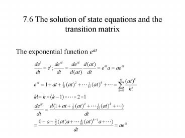
7.6 The solution of state equations and the
transition matrix

• The exponential function eat

2
7.6 The solution of state equations and the
transition matrix

• The matrix exponential eAt is defined as

3
7.6 The solution of state equations and the
transition matrix

4
7.6.1 The transition matrix

• For a given continuous system,
• we can obtain the solution as the follow.
• First, we can re-write the equation as

5
7.6.1 The transition matrix

• Pre-multiplying both sides of the above equation
  by e-At, we obtain
• Integrating the preceding equation between 0 and
  t gives

6
7.6.1 The transition matrix

• Or
• Pre-multiplying both sides by eAt, we have

7
7.6.1 The transition matrix

• That is
• Suppose the input is zero, at time t0 we have

8
7.6.1 The transition matrix

• The solution of the state equation starting with
  the initial condition X(t0) is

9
7.6.1 The transition matrix

• The output of the system is
• The matrix eAt?(t) is called as Transition
  Matrix.

10
7.6.2 Properties of the transition matrix

• Given the transition matrix ?(t) eAt, then
• ,

11
7.6.3 Calculation of the transition matrix

• As
• apply Laplace transform to the above equations,
  we have

12
7.6.3 Calculation of the transition matrix

• Finally we have
• That means we can use inverse Laplace transform
  to calculate the transition matrix.

13
7.6.4 Examples of the transition matrix
calculation

• Example 1 Given the transfer function of a
  system as the follow,
• find its transition matrix?(t).

14
7.6.4 Examples of the transition matrix
calculation

• First, find its state equations,
• then,

15
7.6.4 Examples of the transition matrix
calculation

• Next, find the inverse,

16
7.6.4 Examples of the transition matrix
calculation (cont)

• Finally, calculate the transition matrix,

17
7.7 State variable feedback

• For a continuous-time system given by,
• suppose that all the state variables are
  accessible, a new feedback scheme state
  variable feedback can be implemented.

18
7.7 State variable feedback

u(t)
r(t)
y(t)
X(t)
C

-
KT
19
7.7 State variable feedback

• How does this closed loop system
  behave?where u(t)r(t)-KTX(t), KTk1 k2...
  kn.

20
7.7 State variable feedback

• Substitute u(t) into the above state equations,
  we have

21
7.7 State variable feedback

• For these state equations, we can find the
  transfer function as

22
7.7 State variable feedback

• Example 2 Given the system transfer function as
• suppose a state variable feedback scheme is
  implemented for this system, find its closed loop
  transfer function and draw a diagram to show the
  implementation.

23
7.7 State variable feedback

• First, find its state equations A, B and C.

24
7.7 State variable feedback

• According to the controllable canonical form, we
  obtain
• where

25
7.7 State variable feedback

• Then the closed loop transfer function is

26
7.7 State variable feedback

• Finally we have
• This means that the characteristic equation roots
  may be placed anywhere in the s-plane by choice
  of state variable feedback coefficients.

27
7.7 State variable feedback

• The implementation is shown as the follow

r(t)
y(t)
X(t)
C

-
KT
28
7.7 State variable feedback

• First, the original system can be implemented as
  the follow

x3
e(t)
x2
y(t)
x1

u(t)
?
?
a
?
?
-5
-4
29
7.7 State variable feedback

• Then, the system with state variable feedback can
  be implemented as the follow

-k3
x2
x3
x1
y(t)

r(t)
u(t)
?
?
?
?
?
a
-5
-4
-k2
-k1
30
7.8 Transition matrix for discrete-time state
equations

• For a discrete-time system,
• we will present the solution by a recursion
  procedure and then by the z-transform method.
  Finally, we discuss methods for computing
  (zI-A)-1.

31
7.8.1 Solving discrete-time state equations

• The solution for any positive k may be obtained
  directly by recursion, as follows

32
7.8.1 Solving discrete-time state equations

• By repeating this procedure, we obtain
• Clearly, X(k) consists of two parts, one
  representing the contribution of the initial
  state X(0) and the other the contribution of the
  input u(j), where j0,1,2,k-1. The output y(k)
  is given by y(k)CX(k).

33
7.8.1 Solving discrete-time state equations

• Notice that it is possible to write the solution
  as the follow if the input is zero.
• as
• where ?(k) is a unique n?n matrix satisfying the
  condition

34
7.8.1 Solving discrete-time state equations

• Therefore, we obtain the Transition Matrix for
  discrete-time systems. This transition matrix
  contains all the information about the free
  motions of the system from initial conditions.
  Based on the transition matrix, we can re-write
  X(k) as

35
7.8.2 Computing of transition matrix using
z-transform

• Consider the discrete-time system described as
  the follow
• Applying the z-transform of both sides of the
  above equation, we get

36
7.8.2 Computing of transition matrix using
z-transform

• Applying the inverse z-transform of both sides of
  the above equation, we get
• Comparing the above equation with
• We obtain

37
7.8.2 Computing of transition matrix using
z-transform

• Example Obtain the transition matrix of the
  following discrete-time system
• Solution find the state equations,

38
7.8.2 Computing of transition matrix using
z-transform

• That is
• As
• therefore, we need to find out the inverse

39
7.8.2 Computing of transition matrix using
z-transform

• That is

40
7.8.2 Computing of transition matrix using
z-transform

• The transition matrix ?(k) is now obtained as the
  follows

41
7.8.2 Computing of transition matrix using
z-transform

• That is

42
7.8.2 Computing of transition matrix using
z-transform

• Assume that the initial state is given by
• And the input is unit step function, find the
  y(k).
• Solution Substitute transition matrix into the
  formula below, we have

43
7.8.2 Computing of transition matrix using
z-transform
44
7.8.3 State variable feedback control
For a discrete-time system given by, suppose
that all the state variables are accessible, a
new feedback scheme state variable feedback can
be implemented.
45
7.8.3 State variable feedback
46
7.8.3 State variable feedback
How does this closed loop system
behave?where u(k)r(k)-KTX(k), KTk1 k2...
kn.
47
7.8.3 State variable feedback
Substitute u(k) into the above state equations,
we have
48
7.8.3 State variable feedback
For these state equations, we can find the
transfer function as
49
Tutorial

• Exercise1 Given system differential equation as
  below,
• Suppose the state variables are chosen as
  x1(t)?(t) and x2(t)d?(t)/dt, find out
• The state equations.
• The state equations in form of A, B C.
• The system transfer function using A, B C.
• The transition matrix ?(t)

50
Tutorial

• Solution As x1(t)?(t), x2(t)d?(t)/dt and
• we have

51
Tutorial
A, B and C
52
Tutorial
System transfer function
53
Tutorial
Transition matrix
54
Tutorial
Exercise 2 Given find the transition
matrix?(t) (answer is on study book page 7.24).
55
7.9 Derivation of discrete models from continuous
ones

• For a given continuous-time system,
• we can obtain the solution as the follow.

56
7.9 Derivation of discrete models from continuous
ones

• For a given discrete-time system,
• we can obtain the solution as the follow.

57
7.9 Derivation of discrete models from continuous
ones

• If given a continuous-time system in state
  equation form, you are required to design a
  computer controlled system. Or other way around,
  given a discrete-time system, you are looking for
  the output in continuous-time domain. In these
  cases, how can you manage that?
• Direct derivation
• Via transfer function
• Other methods

58
7.9.1 Discrete-time system with ZOH

• As for the continuous-time system
• During the sample interval
• So that

59
7.9.1 Discrete-time system with ZOH

• Now make a change of variable in the integral
  that is, let
• so that
• when
• and when
• This changes the solution to

60
7.9.1 Discrete-time system with ZOH

• Then we have the discrete-time solution
• As we know that
• Therefore is the plant matrix,
• the driving matrix, and C is the connection
  matrix as the continuous one.

61
7.9.2 Steps of discrete model derivation

• 1. Derive the continuous state equations
• 2. Compute
• then

62
7.9.2 Steps of discrete model derivation

• 3. Compute
• 4. Finally we have

63
7.9.3 Examples of discrete model derivation

• Example Derive the discrete-time system
  corresponding to the following continuous-time
  system when a ZOH circuit is used.
• Notice Suppose there is a ZOH if not given.

64
7.9.3 Examples of discrete model derivation

• 1. Derive the continuous-time state equations
• Applying Laplace transform to the both sides of
  the differential equation.

65
7.9.3 Examples of discrete model derivation

• Write the state equations in controllable
  canonical form
• That is

66
7.9.3 Examples of discrete model derivation

• 2. Compute eAt and eAT

67
7.9.3 Examples of discrete model derivation

• 2. Compute eAt and eAT.

68
7.9.3 Examples of discrete model derivation

• 3. Compute ?.

69
7.9.3 Examples of discrete model derivation

• 4. Finally we have

70
7.9.3 Examples of discrete model derivation

• Example Obtain the discrete-time state and
  output equations and the transfer function of the
  following continuous-time system (T1)

71
7.9.3 Examples of discrete model derivation

• Write the continuous-time state equations in
  controllable canonical form

72
7.9.3 Examples of discrete model derivation

• Compute eAt and eAT

73
7.9.3 Examples of discrete model derivation

• Compute ?

74
7.9.3 Examples of discrete model derivation

• Finally we have
• As T1

75
7.9.3 Examples of discrete model derivation

• The transfer function

76
7.9.4 Other approaches to the discretization

• The same transfer function can be obtained by
  taking z-transform of G(s) when it is preceded by
  a sampler and ZOH.

77
7.9.4 Other approaches to the discretization

• Matlab has a convenient command to discretize the
  continuous-time state equation
• into
• The command is
• ?,?c2d(A, B, T)

78
7.9.4 Other approaches to the discretization

• Example
• A0 10 -2
• B01
• Ad,Bdc2d(A,B,1)
• Ad 1.0000 0.4323
• 0 0.1353
• Bd 0.2838
• 0.4323

79
Reading

• Study book
• Module 7 State space and transition matrix (Page
  7.1 to 7.16)

80
Exercise

• Exercise 1 Given a continuous-time system as
  below,
• if this system is sampled with T1 sec, represent
  the sampled system in the form as