
Process Optimisation - PowerPoint PPT Presentation
1 / 15
Title:
Process Optimisation
Description:
Process model that is used in Process Optimisation relates inputs of the process ... fact that the optimal solution for this type of problem will be located at one ... – PowerPoint PPT presentation
Number of Views:102
Avg rating:3.0/5.0
Title: Process Optimisation
1
Process Optimisation
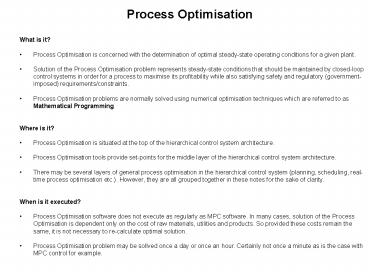
- What is it?
- Process Optimisation is concerned with the
determination of optimal steady-state operating
conditions for a given plant. - Solution of the Process Optimisation problem
represents steady-state conditions that should be
maintained by closed-loop control systems in
order for a process to maximise its profitability
while also satisfying safety and regulatory
(government-imposed) requirements/constraints. - Process Optimisation problems are normally solved
using numerical optimisation techniques which are
referred to as Mathematical Programming. - Where is it?
- Process Optimisation is situated at the top of
the hierarchical control system architecture. - Process Optimisation tools provide set-points for
the middle layer of the hierarchical control
system architecture. - There may be several layers of general process
optimisation in the hierarchical control system
(planning, scheduling, real-time process
optimisation etc.). However, they are all grouped
together in these notes for the sake of clarity.
2
General Features of Process Optimisation Problem
- There are 3 main features of the Process
Optimisation problem all of which are also found
(with some modification) in MPC Control problem. - 1. Cost Function
- Cost function that is used in Process
Optimisation relates directly to the economic
objectives of the process. - Cost function may be linear or nonlinear
depending on a particular situation.. - 2. Process Model
- Process model that is used in Process
Optimisation relates inputs of the process to the
outputs of the process (just like a prediction
model in the case of MPC control). - However, Process Optimisation models are
generally applicable to steady-state rather than
dynamic behaviour of a process. - Process models may be linear or nonlinear
depending on a particular situation.
3
Process Optimisation Example
Background Company owns two production
facilities, both of which produce the same
product but using two different raw
materials. Production facility Plant_A uses
raw material A to produce product C. Production
capacity of Plant_A is 100 tons per
day. Production facility Plant_B uses raw
material B to produce product C. Production
capacity of Plant_B is 200 tons per day. Cost of
raw material A is equal to 30/ton. Cost of raw
material B is equal to 40/ton. Market price
of product C is equal to 50/ton. Current demand
for product C is 120 tons per day. Objective F
ind amounts of A and B that should be consumed
per day in order to maximise profit of a
company. Notation q(X)qunatity of X produced
per day -gtq(C)120. p(X)price of X per ton
-gtp(A)30, p(B)40, p(C)50.
4
Process Optimisation Example
Cost Function Cost function J should represent
profit of a company and can generally be defined
as Profit (Prices of products Amounts of
products) (Costs of raw materials Amounts of
raw materials) In this particular example, our
cost function is given as J p(C) q(C)
p(A) q(A) p(B) q(B) J 50 q(C)
30 q(A) 40 q(B) Process Model Process
model relates quantity of C produced to the
quantities of A abd B consumed. In this example,
it is assumed that 1 ton of either A or B
produces 1 ton of C q(C) q(A)
q(B) Constraints Constraints are imposed to
reflect capacity limits of production facilities
and to reflect market demand. Quantity of
product produced is limited by market demand 0
lt q(C) lt 120 Quantities of A and B consumed
are limited by capacities of production
facilities 0 lt q(A) lt 100 0 lt q(B) lt
200 (lt means smaller than or equal to)
5
Process Optimisation Example
Optimisation Problem max J 50 q(C) 30
q(A) 40 q(B) Subject to q(C) q(A)
q(B) 0 lt q(A) lt 100 0 lt q(B) lt 200 0 lt
q(C) lt 120
6
Process Optimisation Example
Solution First of all let us express cost
function in terms of q(A) and q(B) only J 50
q(A) 50 q(B) 30 q(A) 40 q(B)
J 20 q(A) 10 q(B) Also, let us express
constraint imposed on q(C) in terms of q(A) and
q(B) only 0 lt q(C) lt 120 0 lt q(A) q(B) lt
120
7
Process Optimisation Example
Solution Now we can draw a graph that
pictorially represents constraints for this
optimisation problem
q(A)q(B)120
q(A)100
q(A)q(B)0
q(A)0
q(B)0
q(B)200
8
Process Optimisation Example
Solution For a type of problems that consist
of linear constraints, linear process model and
linear cost function (such as the one defined in
this particular problem), it is relatively easy
to find optimal solution. First of all, define
region within which all of the constraints are
satisfied. In this particular example, such
region is coloured in pale blue colour in the
figure below. This region represents all of the
candidate (i.e. possible) solutions. One of these
solutions is going to be optimal one (i.e. the
best).
q(A)q(B)120
q(A)100
q(A)q(B)0
q(A)0
q(B)0
q(B)200
9
Process Optimisation Example
Solution It is a well-known fact that the
optimal solution for this type of problem will be
located at one of the corners of this region. So
the next step involves calculating value of J at
each of the corners of this region
q(A)100, q(B)20 J 20 100 10 20 2200
q(A)100, q(B)0 J 20 100 10 0 2000
q(A)0, q(B)120 J 20 0 10 120 1200
q(A)0, q(B)0 J 20 0 10 0 0
10
Process Optimisation Example
In this particular case, it was found that
the optimal values of q(A) and q(B) were q(A)100
tons/day and q(B)20 tons/day resulting in a
profit of J 2200 per day
q(A)100, q(B)20 J 20 100 10 20 2200
q(A)100, q(B)0 J 20 100 10 0 2000
q(A)0, q(B)120 J 20 0 10 120 1200
q(A)0, q(B)0 J 20 0 10 0 0
11
Process Optimisation Mathematical Programming
- Process Optimisation problems are generally
solved using the so-called Mathematical
Programming techniques. - Mathematical Programming represents a branch of
Mathematics that deals with problems of numerical
optimisation. - There are numerous sub-classes of mathematical
programming, which are classified according to
the format of cost function, process model and
constraints - Linear Programming (LP) linear cost function,
linear process model, linear constraints - Quadratic Programming (QP) quadratic cost
function, linear process model, linear
constraints - Nonlinear Programming (NLP) either cost
function, process model or constraints (or all of
them) are given in general nonlinear format - There are many efficient algorithms that solve
Mathematical programming problems and these have
been extensively used since 1940s.
12
Process Optimisation Linear Programming
If the cost function, process model and
constraints are all given in linear form then a
resulting optimisation problem can be solved
using Linear Programming (LP). This is arguably
the simplest type of Mathematical programming and
has been extensively used in industry for the
purposes of process design, real-time
optimisation, planning and scheduling. Many
methods that solve more complex types of
Mathematical Programming problems (such as QP and
NLP problems) work by solving LP problems as
their sub-problems. Example covered in these
notes on previous slides was solved using Linear
Programming approach. Linear Programming
originated during the Second World War in an
attempt to plan expenditures and returns such
that losses to the army are minimised while the
losses to the enemy are maximised.
13
Process Optimisation Quadratic Programming
If the cost function is quadratic while
process model and constraints are given in linear
form then a resulting optimisation problem can be
solved using Quadratic Programming (QP). This
type of problem has been extensively studied in
the field of Optimal Control. Quadratic
Programming is used almost exclusively to solve
Model Predictive Control problems.. QP problems
can be efficiently solved in minimal time. This
has allowed proliferation of MPC technology.
14
Process Optimisation Nonlinear Programming
In the case where one or more of the three key
ingredients of the optimisation problem (cost
function, process model, constraints) are
expressed using general nonlinear expressions,
resulting optimisation problem is solved using
Nonlinear Programming (NLP). Nonlinear
Programming problems can be much more difficult
to solve than LP or QP problems. One big issue
that arises when dealing with nonlinear
descriptions of cost function, process model and
constraints is the non-convexity. Such
non-convexity results in the existence of
multiple local optimal points. More specifically,
if the optimisation problem is not convex then
there is no guarantee that the solution of the
NLP problem is indeed optimal. The issue of
multiple local optima is illustrated on the
following slide.
15
Process Optimisation Nonlinear Programming
global maximum
local maxima
local minima
global minimum
Recommended
CrystalGraphics Presentations


![Target Process: DMJ [DRAFT] PowerPoint PPT Presentation](https://s3.amazonaws.com/images.powershow.com/8063781.th0.jpg?_=20160819092)


