Chapter 5 Probability

1
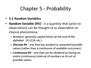
Chapter 5 - Probability

• 5.1 Random Variables
• Random Variable (RV) - is a quantity that (prior
  to observation) can be thought of as dependent on
  chance phenomena.
• Notation generally capital letters at the end of
  the alphabet (X,Y,Z,W, etc.)
• Discrete RV - one that has isolated or separated
  possible values (rather than a continuum of
  available outcomes).
• Continuous RV - one that can be idealized as
  having an entire (continuous) interval of numbers
  as its set of possible values

2
Example 5.1

• Example of a discrete RV
• Let X number of heads in 10 flips of a coin
• Possible values of X are 0, 1, 2, , 10
• Example of a continuous RV
• Let Y weight of babies born at a given hospital
• Possible values of Y are any number between 0 and
  25 lbs.(largest baby was 23 lbs . 12 oz.)

3
Probability Mass Function

• Probability Mass Function (pmf) - for a discrete
  random variable X, having possible values
  is a nonnegative function ,
  with giving the probability that X
  takes the value .
• is in the interval (0,1) for all x.
• The values of sum to 1 when taken at
  all possible values of x.
• So where X is a
  random variable and x is a specific numeric
  value.
• reads as f(x) equals the probability that X
  equals x

4
Example 5.2

• Let Xthe number of goals scored by a hockey team
  in each of their first 9 games
• Suppose a team has X1, 1, 0, 5, 0, 2, 8, 4, 1
  goals.
• Find f(x)

5
Example 5.2

• Graph f(x).

1/3
2/9
1/9
0
2
8
6
4
6
Example 5.2

• Find an

7
Cumulative Density Function

• Cumulative Density Function (cdf) - or cumulative
  probability function for a RV X is a function
  that for each number x gives the
  probability that X takes that value or a smaller
  one.
• Notation
• Find

8
Example 5.3

• Graph

1
2/3
1/3
0
2
8
6
4
9
Example 5.3

• Find F(2.9)

10
Expected Value (Mean)

• Expected Value or Mean of a discrete RV X is
  defined as
• Often denoted µ
• Find EX (from example 5.2)

11
Variance and Standard Deviation

• Variance - of a discrete random variable X is
  defined as
• Often denoted s2
• Standard Deviation of X is
• Often denoted s

12
Example 5.4

• Find Var(X) and SD(X)

13
Common Discrete Distributions

• We will explore some common discrete
  distributions
• Binomial Distribution
• Geometric Distribution
• Poisson Distribution
• Assumptions for many discrete distributions
• Independent, identical, success/failure trials
• Constant chance of success on each repetition of
  the scenario (call the probability of success p).
• Repetitions are independent in the sense that
  knowing the outcome of any one of them does not
  change assessments of chance related to any
  others.

14
Binomial Distribution

• Suppose we have n trials, with success
  probability of each trial being p.
• X the number of successes in n independent,
  identical trials
• Then X has the binomial(n, p) distribution.
• Denoted
• pmf for n a positive integer and 0ltplt1.

15
Binomial pmf Properties

• Factorials
• Example
• When plt0.5 the histogram for f(x) is
  right-skewed.
• When pgt0.5 the histogram for f(x) is left-skewed.
• When p0.5 the histogram is symmetric.

16
Binomial pmf Explanation

• Probability of success is p, so probability of
  failure is (1 p).
• There are x successes and n x failures.
• The order in which the successes and failures
  occur doesnt matter, so there are many
  combinations (n choose x).

17
Binomial Expectations

• Mean of Bin(n,p)
• Variance of Bin(n,p)

18
Example 5.5

• A multiple choice quiz has 10 questions each with
  4 alternatives. A student forgot to study and
  wished to get at least 3 correct. What is the
  probability this will occur if he guesses on
  every question?

19
Example 5.5
20
Example 5.5

• What is the probability that he gets 9 or more
  correct?

21
Example 5.5

• Find EX, Var(X), and SD(X)

22
Geometric distribution

• p probability of success
• X number of trials required to obtain the first
  success
• Then, X has geometric distribution with parameter
  p.
• Denoted
• pmffor 0ltplt1.

23
Geometric pmf Explanation

• The Geo pmf is the probability of the first
  success on trial x.

24
Geometric Expectations

• Mean of Geo(p)
• Variance of Geo(p)

25
Example 5.6

• We know that when throwing a fair die, the
  probability of rolling a 2 is 1/6. What is the
  probability that when continuing to roll a die we
  see a 2 for the first time on the 5th roll?

26
Example 5.6

• What is the probability that the first 2 appears
  after the 2nd roll?

27
Example 5.6

• Find EX and Var(X)

28
Poisson Distribution

• Used to describe random counts of the number of
  occurrences of a relatively rare phenomenon
  across a specified interval of time or space.
• X the number of occurrences of a rare event
• X has the Poisson distribution with parameter ?.
• Denoted
• pmffor ? gt 0

29
Poisson Explanation

• What is the parameter ??
• Suppose we have a Bin(n, p) distribution with
  extremely small success probability p and large
  n.
• We use the Pois(?) distribution to approximate
  the Bin(n, p), where we let ? np.
• Example
• X of people out of 10 who go through checkout
  5 at a Hy-Vee during a 5 minute span.
• X of people in the store who go through
  checkout 5 at a Hy-Vee during a 5 minute span.

30
Poisson Expectations

• Mean of Pois(?)
• Variance of Pois(?)

31
Example 5.7

• Public health records over 5 years found 286
  diagnosed cases of leukemia out of 1,152,695
  children under age 15. What is the probability
  that in a town of size 7076, wed find 2 or more
  cases of leukemia over 5 years?

32
Example 5.7
33
Example 5.7

• What is the expected number of leukemia cases
  (over a 5 year span) for this town?

34
5.2 Continuous RVs

• Recall
• Continuous RV - one that can be idealized as
  having an entire (continuous) interval of numbers
  as its set of possible values
• Concepts of pmf, cdf, EX, VarX, are similar to
  discrete, but now over a continuous interval.
• Under continuous data, we have a pdf instead of
  pmf
• We evaluate over intervals instead of discrete
  values

35
Probability Density Function (pdf)

• Probability Density Function (pdf) for a
  continuous RV X is a nonnegative function f(x)
  such that for all ab,with the added
  constraint
• For a continuous RV,
  for all values of x because
• Calculus area under the curve f(x)

36
Example 5.8

• Problem 1 from the Section 2 Exercises, page 263
• Suppose a RV X has pdf
• Find k.

37
Example 5.8

• Sketch the pdf f(x).

1.0
0.5
0.5
1.0
38
Example 5.8

• Evaluate

39
CDF for Continuous RV

• Cumulative Density Function (cdf) for a
  continuous RV X is given by
• To obtain f(x) from F(x),

40
Example 5.9

• (Continued from ex. 5.8) Compute the cdf of X.

41
Example 5.9

• (Continued from ex. 5.8) Graph the cdf of X.

42
Expectations

• Mean of a continuous RV X is given by
• Variance of a continuous RV X is given by

43
Example 5.10

• (Continued from ex. 5.8) Calculate EX

44
Example 5.10

• (Continued from ex. 5.8) Calculate SD(X)

45
Common Continuous Distributions

• We will explore some common continuous
  distributions
• Normal Distribution
• Exponential Distribution
• Assumptions for many continuous distributions
• Probability of any single observation is zero
  (PXx0).
• Repetitions are independent in the sense that
  knowing the outcome of any one of them does not
  change assessments of chance related to any
  others.

46
Normal Distribution

• Normal Distribution with parameters µ and s2 is
  a continuous distribution with pdffor any
  real number µ and s gt 0.
• Denoted

47
Properties of the Normal Dist.

• For , EX µ, and
  Var(X) s2
• The graph of the normal pdf is bell-shaped,
  symmetric about µ, with inflection points at µ
  s and µ - s.

f(x)
x
µ - 2s
µ - s
µ
µ s
µ 2s
48
Standard Normal Distribution

• Standard Normal Distribution is a special case
  of the normal distribution where µ0 and s1.
• Denoted
• It is often easier to work with N(0,1) so if we
  have data that is N(µ,s), we can perform a
  transformation to get N(0,1).
• Table B.3 (p.788) gives the values for the cdf of
  the N(0,1).
• Margins are values of z
• Body gives values of
• Example PZ -1.32 .0934

49
Transform to N(0,1)

• Given we can transform
  the variable by the following
• This results in
• Example

50
Useful Equalities for N(0,1)

• PZ a PZ -a 1 - PZ a
• Pa Z b PZ b - PZ a
• Pa Z PZ a PZ -a 2PZ -a
• PZ a P-a Z a PZ a - PZ -a
  1 - 2PZ -a

51
Useful Equality 1 for N(0,1)
52
Useful Equality 2 for N(0,1)
53
Useful Equality 3 for N(0,1)
54
Useful Equality 4 for N(0,1)
55
Example 5.11

• Let . Find the following.
• PZ 2.12
• P-0.32 Z 1.54

56
Example 5.11

• PZ 0.79
• PZ 0.93

57
Example 5.11

• Find the value of c.
• PZ c 0.90
• PZ c 0.90

58
Example 5.12

• Let .
• Find PX lt 45.2

59
Example 5.12

• Find PX 43 2.0

60
Example 5.12

• If PX c 0.30, find c.

61
Exponential Distribution

• Exponential Distribution is a continuous
  probability distribution useful for describing
  waiting times until occurrences.
• Exponential distribution with parameter agt0 has
  pdf
• Denoted

62
Graph of Exponential pdf
f(x)
x
63
Exp(a) cdf and Expectations

• Given , the cdf is the
  following
• The expectations are the following

64
Example 5.13

• (p.263 problem 5) The mileage to first failure
  for a model of military personnel carrier can be
  modeled as exponential with mean 1000 miles.
• What is the probability that a vehicle of this
  type gives less than 500 miles of service before
  its first failure?

65
Example 5.13

• What is the probability it gives at least 2000
  miles of service?

66
5.4 Joint Distributions and Independence

• Suppose we have two RVs at the same time.
• First consider discrete case.
• Joint Probability Function (joint pmf) for two
  discrete RVs X and Y, the joint pmf is a
  nonnegative function f(x,y) giving the
  probability that X equals x and Y equals y, at
  the same time.

67
Example 5.14

• Suppose we monitor the first 15 sales of tickets
  to a football game.
• X the number of adult tickets bought in a sale
• Y number of childrens tickets bought in a
  sale
• Suppose that the ordered pairs (x,y) from 15
  sales are(2,0), (2,1), (3,0), (3,1), (1,2),
  (1,1), (4,0), (4,1), (2,0), (2,0), (3,1), (2,0),
  (1,2), (2,1), (2,1)

68
Example 5.14
- Find f(x,y)
Y
X
Note table sums up to 1.
69
Example 5.14

• Find PXgtY

70
Marginal Probability Function

• Marginal Probability Function given two
  discrete RVs (X,Y), the marginal probability
  functions are defined as
• Note that fX(x) is just like f(x) from section
  5.1.

71
Example 5.15

• (Continued from ex. 5.14) Find fX(x) and fY(y).

72
Conditional Distribution

• Conditional probability function for discrete
  random variables X and Y with joint probability
  function f(x,y), the conditional probability
  function of X given Y y is the function of
  x and the conditional probability function of
  Y given X x is the function of y

73
Example 5.16

• (Continued from ex. 5.14) Suppose that we know a
  sale consists of 1 childrens ticket. What are
  the probabilities that X1, that X2, that X3,
  and that X4?

74
Example 5.16

• What is the probability that 2 childrens tickets
  are sold given that 1 adult ticket is sold?

75
Independence

• Independence discrete random variables X and Y
  are called independent if their joint pmf,
  f(x,y), is the product of their marginal
  probability functions.
• If this equality does not hold, then X and Y are
  dependent.
• Only need to find one example to prove dependence.

76
Example 5.17

• (Continued from ex. 5.14) Are X and Y independent?

77
Example 5.18

• Suppose a coin is flipped twice. Let X0 if the
  first flip is a heads and 1 if it is tails. Let
  Y0 if the second flip is head and 1 if it is
  tails. Then we have the following table

Y
f(x, y)
X
78
Example 5.18

• Find fX(x) and fY(y).

79
Example 5.18

• Are X and Y independent?

80
Independent and Identically Distributed (iid)

• Independent and Identically Distributed random
  variables X1, X2, , Xn all have the same
  marginal distribution and are all independent of
  one another
• Example
• Suppose we have 5 separate batches of 100 bolts
  in which 2 in each batch are defective.
• If Xi the number of defective bolts when 10 are
  drawn from batch i, then X1, X2, X3, X4, X5 are
  iid Bin(10, .02).
• This is because each Xi itself is Bin(10, .02),
  and because the outcomes from each batch are
  independent from the other batches.

81
Jointly Continuous RVs

• Joint probability function (joint pdf) for
  continuous RVs X and Y, is a nonnegative
  function f(x,y) such that for any region
  Rand with

82
Example 5.19

• Suppose a pair of random variables have the joint
  pdf
• Prove that this is a valid pdf.

83
Example 5.19

• Find PX 2Y 1

84
Example 5.19
85
Example 5.19 - Illustration
86
Example 5.19

• Find PX gt 1/2

87
Example 5.19 - Illustration
88
Marginal pdfs and Independence

• Marginal probability function given two
  continuous RVs (X,Y), the marginal pdfs are
  defined as
• Independence continuous random variables X and
  Y are independent if

89
Example 5.20

• (Continued from ex. 5.19) Find fX(x) and fY(y).

90
Example 5.20

• Are X and Y independent?

91
Conditional pdf

• Conditional pdf for continuous random variables
  X and Y with joint probability function f(x,y),
  the conditional pdf of X given Y y is the
  function of x and the conditional pdf of Y
  given X x is the function of y

92
Example 5.21

• (Continued from ex. 5.19) Find the conditional
  pdf of X given Y y.
• Note When independence holds, the following are
  true.

93
5.5 Functions of Several RVs

• Given the joint distribution of RVs X, Y, , Z,
  what can we say about U g(X,Y,,Z) (a function
  of the RVs)?
• Often, a function of RVs is itself a RV.
• Sometimes the distribution of U is too
  complicated to calculate analytically
• Read section 5.5.2 for more info (p.304-307)
• Common functions
• Linear g(X,Y,Z) XYZ
• Product g(X,Y,Z) XYZ

94
Example 5.22

• Consider the ticket information for example 5.14.
  Suppose now that we arent interested in the
  breakdown into child and adult tickets, but care
  about only the total number of tickets sold in
  each sale. In other words, we are interested in
  UXY. So, here g(X,Y)XY.
• Find the pmf for the random variable U.

95
Expectations for Linear Functions of RVs

• Suppose that X,Y,,Z are n independent random
  variables and that a0, a1, , an are n1
  constants. Define the random variable U as the
  following linear combination of X,Y,,Z
• Then,
• Note Independence is necessary for the Variance
  property, but not for the Mean property.

96
Example 5.23

• Let X,Y, and Z be three independent RVs with the
  following means and standard deviations
• Define U 2 3X 4Z - Y

97
Example 5.23

• Find EU.

98
Example 5.23

• Find SD(U).

99
Expectations of iid RVs

• Suppose that X1, X2, , Xn are n iid random
  variables with common mean µ and common variance
  s2. Define the random variable as the average
  of these
• Then

100
Proof 1
101
Proof 2
102
Propagation of Error Formulas(Delta Method)

• Used when Ug(X,Y,,Z) is not a linear function.
• If X,Y,,Z are independent random variables, for
  small enough variances Var X,,Var Z, the random
  variable Ug(X,Y,Z) has approximate meanand
  approximate variance

103
Example 5.24

• Suppose that X,Y, and Z are independent RVs with
• Define

104
Example 5.24

• Find the approximate expected value of U.

105
Example 5.24

• Find the approximate variance of U.

106
Central Limit Theorem

• If X1, X2, , Xn are iid random variables (with
  mean µ and variance s2), then for large n, the
  random variable is approximately normally
  distributed.
• Specifically,
• Rule of Thumb n 25 is large

107
Example 5.25

• Suppose that X1, X2, , X40 are iid Bin(12,
  0.6).
• Find and .

108
Example 5.25

• Find