Market Risk VAR

1
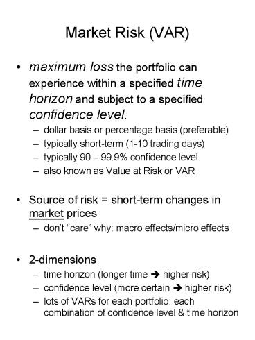
Market Risk (VAR)

• maximum loss the portfolio can experience within
  a specified time horizon and subject to a
  specified confidence level.
• dollar basis or percentage basis (preferable)
• typically short-term (1-10 trading days)
• typically 90 99.9 confidence level
• also known as Value at Risk or VAR
• Source of risk short-term changes in market
  prices
• dont care why macro effects/micro effects
• 2-dimensions
• time horizon (longer time ? higher risk)
• confidence level (more certain ? higher risk)
• lots of VARs for each portfolio each combination
  of confidence level time horizon

2
Market Risk (VAR)

• Time horizon
• No time horizon?
• infinite time ? 100 loss is possible
• anything that can happen, will happen
• Related to liquidity of position
• how quickly can you get out if things go bad?
• Related to institutional reaction speed
• how quickly will you get out if things go bad?
• Confidence level
• No confidence level?
• absolute certainty ? 100 loss is possible (e.g.,
  nuclear war)
• 100 confidence level how often wrong
• Related to need for certainty
• regulatory requirements
• job security
• preferences/tastes/risk aversion

3
Simple Example

• Daily portfolio return determined by flipping a
  coin.
• heads 1 tails -1 ? ER 0
• 10-day horizon, 95 confidence
• VAR -4
• you will be wrong (bigger loss) 5.47 of time.

4
Interpretation of VAR

• If the 3-day VAR of my 50 million portfolio is
  1.6 million (3.2) with 99 confidence, then
• over the next 3 days, there is only a 1 chance
  that my portfolio will lose more than 1.6
  million.
• during the next one hundred 3-day periods (300
  days total), my portfolio will likely lose more
  than 1.6 million during one of them.
• The focus of market risk (VAR) is usually on the
  first interpretation. The near future.

5
Uses of Market Risk (VAR)

• Trading Portfolio head trader
• short-term focus
• liquid securities
• see total risk across traders/positions
• set risk (capital) limits per trader
• evaluate trading performance relative to the
  capital at risk
• Banking
• regulatory concerns
• Basel standards
• Tail risk
• more generalized concern about worst possible
  outcomes as a measure of risk
• alternative to standard deviation and similar
  measures of risk

6
Estimating of Market Risk

• 2 types of approach
• historical
• parametric
• Historical approaches
• assume returns in the near future will follow the
  pattern of the recent past
• measure worst losses from recent past
• Parametric approaches
• assume future returns follow a fixed distribution
• estimate parameters of the distribution
• calculate VAR
• in practice, mathematics is complex

7
Historical Simulation Approach

• Make no assumption about the distribution (or
  shape) of future returns
• Assume that in near future, daily return pattern
  will be similar to recent past
• at least for the next day or two
• Focus on current composition of portfolio
• what assets are held?
• how many/much of each?
• Pretend that the portfolios contents do not
  change
• go back and ask what would this portfolio have
  been worth yesterday?, The day before?, etc.

8
Historical Simulation Approach

• (1) Collect historic security prices
• for each asset in todays portfolio.
• per share/unit price for yesterday, day before,
  etc.
• At least 200 days back, probably more.
• (2) Calculate daily portfolio values
• for each previous day
• assume portfolio composition was the same as
  today (adjusted for splits, dividends, etc.)
• calculate number of shares/units times price per
  share/unit
• Example
• 201 days of historic prices
• 1-day time horizon
• 95 confidence level

9
Historical Simulation Approach

• (3) Calculate daily percentage changes in
  portfolio values
• (PVt PVt-1) PVt-1
• 201 days ? 200 changes in value
• (4) Sort daily percentage changes in portfolio
  value
• highest (positive) to lowest (negative)
• (5) Calculate VAR
• measure cut off for selected confidence level
• separate 10 (5) worst from 190 (95) best
• typically use average of 10th and 11th worst
  returns (midpoint of separation)

10
Historical Simulation Approach

• Another example
• 601 days of historic price data (250 days 1
  trading year)
• 2-day time horizon
• 99 confidence level
• Measure portfolio value for each day
• Calculate 2-day percentage changes in portfolio
  value
• (PVt PVt-2) PVt-2
• do not use overlapping periods
• day -2 ? day 0, day -4 ? day -2, etc.
• not day -3 ? day -1 (which would overlap)
• 601 days ? 300 changes in value

11
Historical Simulation Approach

• Sort 2-day percentage changes in portfolio value
• highest (positive) to lowest (negative)
• Calculate VAR
• measure cut off for selected confidence level
• separate 3 (1) worst from 297 (99) best returns
• typically use average of 3rd and 4th worst 2-day
  returns (midpoint of separation)

12
Historical Simulation Approach

• Advantages
• simple computation
• no distribution assumptions
• Disadvantages
• trusting the historical data
• past is like the future?
• not a violation of efficient markets
• hard to measure high confidence levels (e.g.,
  99.9) too much data required
• hard to measure longer time horizons (e.g., 5
  days or 10 days) too much data required
• what do you do about
• new securities?
• non-traded securities?
• infrequently-traded securities?

13
Parametric Approach

• Idea
• make assumption about the way daily returns are
  distributed
• estimate the parameters of the distribution
• calculate VAR from the distribution
• recall our coin flipping example
• Normal Distribution
• a.k.a. bell curve
• common distributional assumption
• symmetric
• 2 parameters
• mean (µ) which is the expected value
• standard deviation (s) higher is riskier

14
Normal Distribution2 Parameters
s
µ
The area under the curve equals 100
15
Normal Distribution2-tailed confidence intervals
µ
µs
µ-s
µ2s
µ3s
µ-2s
µ-3s
68
95
99
16
Normal Distribution1-tailed confidence intervals
1-X Bad Outcomes
X Good Outcomes
µ
µ-???s
How many standard deviations below the mean for
X confidence level?
17
Parametric w/Normal Distribution

• Z-score of standard deviations below mean
  (for given confidence level)
• 90 1.282
• 95 1.645
• 99 2.327
• 99.9 3.090
• VAR µ - (z-score s)
• µ mean portfolio daily return
• s standard deviation of portfolios daily
  returns
• daily return daily percentage price change
• Multiple days
• assume each is independent
• i.i.d. (independently and identically
  distributied) normal
• VAR (N µ) - (vN z-score s)

18
Parametric w/Normal Distribution

• Example
• µportfolio 0.02
• sportfolio 0.17
• 1-day VAR w/99 confidence
• 0.02 - (2.327 0.17)
• 0.38
• 5-day VAR w/95 confidence
• (50.02) - (v5 1.645 0.17)
• 0.53

19
Parametric w/Normal Distribution

• What does the mean mean?
• known return (opposite of risk)
• if positive, dampens (reduces) the market risk
  measure
• if negative, why are you holding the portfolio?
• Many risk managers assume µ 0
• N-day VAR (vN z-score s)
• Redo Examples assuming µ 0
• - 1-day VAR w/99 confidence
• (v1 2.327 0.17)
• 0.40 gt 0.38
• - 5-day VAR w/95 confidence
• (v5 1.645 0.17)
• 0.63 gt 0.53
• A matter of taste

20
Parametric w/Normal Distribution

• How do I estimate parameters for my portfolios
  return distribution?
• multiple assets
• assume a joint normal distribution
• for each asset, need to know
• value of holding in portfolio
• mean daily return (µ)
• standard deviation of daily returns (s)
• correlation of returns with each other asset in
  portfolio (?) -1 ? 1
• Mean daily return of portfolio
• µportfolio ? wj µj.
• wj (PVj/PVportfolio)
• value weighted average
• Variance of daily return of portfolio
• s2portfolio ?j?k wj wk sj sk ?j,k
• sportfolio vs2portfolio.

21
Parametric w/Normal Distribution

• Weights
• wA 30M/50M 0.6
• wB 20M/50M 0.4
• Mean Return
• (0.6 0.03) (0.4 -0.01)
• 0.0140
• Return Variance (s2)
• (.6 .6 .12 .12 1)
• (.6 .4 .12 .20 .35)
• (.4 .6 .20 .12 .35)
• (.4 .4 .20 .20 1)
• 0.0156 (2)
• Standard Deviation (s)
• v0.0156 (2) 0.1249

22
Parametric w/Normal Distribution

• Example continued
• What is the 3-day VAR of this portfolio with
  99.9 confidence
• use calculated mean return
• (30.0140) (v33.0900.1249)
• 0.6265 0.63
• assume mean return 0
• (v33.0900.1249)
• 0.6685 0.67

23
Factor Approach

• Problem with parametric approach
• too many parameters to estimate
• N-asset portfolio requires
• N means
• N standard deviations
• (N N-1)/2 correlations this kills you
• 50 assets ? 1,225 correlations!
• 500 assets ? 124,750 correlations!!!
• 500 asset returns for 500 days only 250,000
  observations
• Factor Approach to Parametric VAR
• select a small set of economic factors that have
  impact on a lot of securities and account for
  most daily price variation
• e.g., interest rates, stock index returns, credit
  spreads, foreign exchange rates, etc.
• determine each assets sensitivity to each factor

24
Factor Approach Step-by-Step

• (1) Select factors
• those that account for most daily price changes
• (2) Make distributional assumption
• joint normal distribution
• (3) Estimate parameter values for factor
  distribution
• µs, ss, and ?s
• (4) Measure the sensitivity of each asset in my
  portfolio to each factor
• called the factor loadings
• (5) VAR weighted sum of the sensitivities to
  each factor multiplied by the maximum change in
  each factor

25
Factor Approach1-factor model

• 1-factor model
• the factor is the short-term interest rate
• Distributional assumption
• i.i.d. normal
• Factor loadings
• each assets modified duration
• Measure maximum interest rate change
• given distribution (µ and s)
• time horizon
• confidence level
• VAR maximum change in value MDportfolio
  maximum ?I
• Using duration model ?PV/PV -MD ?i

26
Factor Approach1-factor model example

• Parameter Values
• µ?i 0.00 (natural assumption)
• s?i 0.22
• VAR requirements
• 4-day time horizon
• 90 confidence level
• Factor loadings
• MDportfolio 2.75 years
• Maximum ?i
• v4 1.282 0.22
• 0.5641
• VAR
• 2.75 0.5641
• 1.5512
• More factors? Much more complicated.

27
VAR Critique

• Benefits
• single number (per time horizon/confidence)
• maximum loss
• flexible
• handles all assets / sources of risk
• focuses on value of portfolio
• related to value of firm
• recognizes benefits of portfolio diversification
• Concerns
• most of the time nature, but its the big
  surprises that kill you
• no consensus on how best to measure
• generally assumes future will be like past
• Parametric Approach
• instability of parameters
• fat tails problem (extreme events occur too
  frequently)