
1'1 What is a signal - PowerPoint PPT Presentation
Title:
1'1 What is a signal
Description:
A signal is formally defined as a function of one or more variables that conveys ... NASA space shuttle launch. (Courtesy of NASA.) 6. Introduction. 1. CHAPTER ... – PowerPoint PPT presentation
Number of Views:36
Avg rating:3.0/5.0
Title: 1'1 What is a signal
1
Introduction
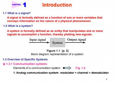
1.1 What is a signal?
A signal is formally defined as a function of one
or more variables that conveys information on the
nature of a physical phenomenon.
1.2 What is a system?
A system is formally defined as an entity that
manipulates one or more signals to accomplish a
function, thereby yielding new signals.
Figure 1.1 (p. 2)Block diagram representation
of a system.
1.3 Overview of Specific Systems
? 1.3.1 Communication systems
Elements of a communication system
Fig. 1.2
1. Analog communication system modulator
channel demodulator
2
Introduction
Figure 1.2 (p. 3)Elements of a communication
system. The transmitter changes the message
signal into a form suitable for transmission over
the channel. The receiver processes the channel
output (i.e., the received signal) to produce an
estimate of the message signal.
? Modulation
2. Digital communication system sampling
quantization coding ? transmitter ? channel ?
receiver
? Two basic modes of communication
Fig. 1.3
- Broadcasting
- Point-to-point communication
Radio, television
Telephone, deep-space communication
3
Introduction
Figure 1.3 (p. 5)(a) Snapshot of Pathfinder
exploring the surface of Mars. (b) The 70-meter
(230-foot) diameter antenna located at Canberra,
Australia. The surface of the 70-meter reflector
must remain accurate within a fraction of the
signals wavelength. (Courtesy of Jet Propulsion
Laboratory.)
4
Introduction
? 1.3.2 Control systems
Figure 1.4 (p. 7)Block diagram of a feedback
control system. The controller drives the plant,
whose disturbed output drives the sensor(s). The
resulting feedback signal is subtracted from the
reference input to produce an error signal e(t),
which, in turn, drives the controller. The
feedback loop is thereby closed.
? Reasons for using control system 1. Response,
2. Robustness
? Closed-loop control system Fig. 1.4.
Controller digital computer (Fig. 1.5.)
- Single-input, single-output (SISO) system
- Multiple-input, multiple-output (MIMO) system
5
Introduction
Figure 1.5 (p. 8)NASA space shuttle
launch.(Courtesy of NASA.)
6
Introduction
Analog Versus Digital Signal Processing
- Digital approach has two advantages over analog
approach - Flexibility
- Repeatability
1.4 Classification of Signals
1. Continuous-time and discrete-time signals
Parentheses (?)
Continuous-time signals x(t)
Fig. 1-11.
where t nTs
Discrete-time signals
(1.1)
Fig. 1-12.
Brackets ?
7
Introduction
Figure 1.11 (p. 17)Continuous-time signal.
Figure 1.12 (p. 17)(a) Continuous-time signal
x(t). (b) Representation of x(t) as a
discrete-time signal xn.
8
Introduction
Symmetric about vertical axis
2. Even and odd signals
Even signals
(1.2)
Odd signals
(1.3)
Example 1.1
Antisymmetric about origin
Consider the signal
Is the signal x(t) an even or an odd function of
time?
ltSol.gt
odd function
9
Introduction
? Even-odd decomposition of x(t)
Example 1.2
Find the even and odd components of the signal
where
ltSol.gt
Even component
(1.4)
(1.5)
Odd component
10
Introduction
? Conjugate symmetric
A complex-valued signal x(t) is said to be
conjugate symmetric if
(1.6)
Refer to Fig. 1-13 Problem 1-2
Let
3. Periodic and nonperiodic signals
(Continuous-Time Case)
Periodic signals
(1.7)
Figure 1.13 (p. 20)(a) One example of
continuous-time signal. (b) Another example of a
continuous-time signal.
and
Fundamental frequency
(1.8)
Angular frequency
(1.9)
11
Introduction
? Example of periodic and nonperiodic signals
Fig. 1-14.
Figure 1.14 (p. 21)(a) Square wave with
amplitude A 1 and period T 0.2s. (b)
Rectangular pulse of amplitude A and duration T1.
? Periodic and nonperiodic signals (Discrete-Time
Case)
(1.10)
N positive integer
Fundamental frequency of xn
(1.11)
12
Introduction
Figure 1.15 (p. 21)Triangular wave alternative
between 1 and 1 for Problem 1.3.
? Example of periodic and nonperiodic signals
Fig. 1-16 and Fig. 1-17.
Figure 1.16 (p. 22)Discrete-time square wave
alternative between 1 and 1.
13
Introduction
Figure 1.17 (p. 22)Aperiodic discrete-time
signal consisting of three nonzero samples.
4. Deterministic signals and random signals
A deterministic signal is a signal about which
there is no uncertainty with respect to its value
at any time.
Figure 1.13 Figure 1.17
A random signal is a signal about which there is
uncertainty before it occurs.
Figure 1.9
5. Energy signals and power signals
Instantaneous power
If R 1 ? and x(t) represents a current or a
voltage, then the instantaneous power is
(1.12)
(1.14)
(1.13)
14
Introduction
Fig. 1.9
15
Introduction
The total energy of the continuous-time signal
x(t) is
? Discrete-time case
Total energy of xn
(1.15)
(1.18)
Time-averaged, or average, power is
Average power of xn
(1.16)
(1.19)
For periodic signal, the time-averaged power is
(1.17)
(1.20)
? Energy signal If and only if the total
energy of the signal satisfies the condition
? Power signal If and only if the average
power of the signal satisfies the condition
16
Introduction
- Energy signal has zero time-average power (why?)
- Power signal has infinite energy (why?)
- Energy signal and power signal are mutually
exclusive - Periodic signal and random signal are usually
viewed as power signal - Nonperiodic and deterministic are usually viewed
as energy signal
17
Introduction
1.5 Basic Operations on Signals
? 1.5.1 Operations Performed on dependent
Variables
c scaling factor
Amplitude scaling
x(t)
(1.21)
Discrete-time case
xn
Performed by amplifier
Addition
(1.22)
Discrete-time case
Multiplication
Ex. AM modulation
(1.23)
Figure 1.18 (p. 26)Inductor with current i(t),
inducing voltage v(t) across its terminals.
Differentiation
Inductor
(1.25)
(1.24)
Integration
(1.26)
18
Introduction
Capacitor
(1.27)
Figure 1.19 (p. 27)Capacitor with voltage v(t)
across its terminals, inducing current i(t).
? 1.5.2 Operations Performed on
independent Variables
Time scaling
a gt1 ? compressed 0 lt a lt 1 ? expanded
Fig. 1-20.
Figure 1.20 (p. 27) Time-scaling operation (a)
continuous-time signal x(t), (b) version of x(t)
compressed by a factor of 2, and (c) version of
x(t) expanded by a factor of 2.
19
Introduction
Discrete-time case
k integer
Some values lost!
Figure 1.21 (p. 28)Effect of time scaling on a
discrete-time signal (a) discrete-time signal
xn and (b) version of xn compressed by a
factor of 2, with some values of the original
xn lost as a result of the compression.
Reflection
The signal y(t) represents a reflected version of
x(t) about t 0.
Ex. 1-3 Consider the triangular pulse x(t) shown
in Fig. 1-22(a). Find the reflected version of
x(t) about the amplitude axis (i.e., the origin).
ltSol.gt Fig.1-22(b).
20
Introduction
Figure 1.22 (p. 28)Operation of reflection (a)
continuous-time signal x(t) and (b) reflected
version of x(t) about the origin.
t0 gt 0 ? shift toward right t0 lt 0 ? shift toward
left
Time shifting
Ex. 1-4 Time Shifting Fig. 1-23.
Figure 1.23 (p. 29)Time-shifting operation (a)
continuous-time signal in the form of a
rectangular pulse of amplitude 1.0 and duration
1.0, symmetric about the origin and (b)
time-shifted version of x(t) by 2 time shifts.
21
Introduction
Discrete-time case
where m is a positive or negative integer
? 1.5.3 Precedence Rule for Time Shifting and
Time Scaling
1. Combination of time shifting and time scaling
(1.28)
(1.29)
(1.30)
2. Operation order
To achieve Eq. (1.28),
1st step time shifting
2nd step time scaling
Ex. 1-5 Precedence Rule for Continuous-Time Signal
Consider the rectangular pulse x(t) depicted in
Fig. 1-24(a). Find y(t)x(2t 3).
ltSol.gt
Case 1 Fig. 1-24. ? Shifting first, then scaling
Case 2 Fig. 1-25. ? Scaling first, then shifting
22
Introduction
Figure 1.24 (p. 31)The proper order in which
the operations of time scaling and time shifting
should be applied in the case of the
continuous-time signal of Example 1.5. (a)
Rectangular pulse x(t) of amplitude 1.0 and
duration 2.0, symmetric about the origin. (b)
Intermediate pulse v(t), representing a
time-shifted version of x(t). (c) Desired signal
y(t), resulting from the compression of v(t) by a
factor of 2.
23
Introduction
Figure 1.25 (p. 31)The incorrect way of applying
the precedence rule. (a) Signal x(t). (b)
Time-scaled signal v(t) x(2t). (c) Signal y(t)
obtained by shifting v(t) x(2t) by 3 time
units, which yields y(t) x(2(t 3)).
Ex. 1-6 Precedence Rule for Discrete-Time Signal
A discrete-time signal is defined by
Find yn x2n 3.
24
Introduction
ltSol.gt See Fig. 1-27.
Figure 1.27 (p. 33)The proper order of applying
the operations of time scaling and time shifting
for the case of a discrete-time signal. (a)
Discrete-time signal xn, antisymmetric about
the origin. (b) Intermediate signal v(n) obtained
by shifting xn to the left by 3 samples. (c)
Discrete-time signal yn resulting from the
compression of vn by a factor of 2, as a result
of which two samples of the original xn,
located at n 2, 2, are lost.
Recommended
CrystalGraphics Presentations


