ARmodels

1
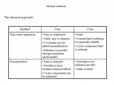
Modern methods The classical approach
2
Explanation to the static behaviour The
classical approach assumes all components except
the irregular ones (i.e. ?t and IRt ) to be
deterministic, i.e. fixed functions or
constants To overcome this problem, all
components should be allowed to be stochastic,
i.e. be random variates. A time series yt
should from a statistical point of view be
treated as a stochastic process. We will
interchangeably use the terms time series and
process depending on the situation.
3
Stationary and non-stationary time series
4
AR-models
Consider the model ytdfyt-1at with at
i.i.d with zero mean and constant variance
s2 Set d0 by sake of simplicity?E(yt )0 Let
R(k)Cov(yt,yt-k ) Cov(yt,ytk )E(yt yt-k )
E(yt ytk ) ? R(0)Var(yt) assumed to be
constant
5
Now R(0)E(yt yt ) E(yt (fyt-1at ) f E(yt
yt-1 ) E(yt at ) fR(1) E((fyt-1at
) at ) fR(1) f E(yt-1 at ) E(at at )
fR(1) 0 s2 (for at is independent of
yt-1 ) R(1)E(yt yt1 ) E(yt (fytat1 ) f
E(yt yt ) E(yt at1 ) fR(0)0
(for at1 is independent of yt ) R(2) E(yt
yt2 ) E(yt (fyt1at2 ) f E(yt yt1 )
E(yt at2 ) fR(1)0 (for
at1 is independent of yt ) ?
6
R(0) fR(1) s2 R(1) fR(0) Yule-Walker
equations R(2) fR(1) ? R(k ) fR(k-1)
fkR(0) R(0) f2 R(0) s2 ?
7
Note that for R(0) to become positive and finite
(which we require from a variance) the following
must hold
This in effect the condition for an AR(1)-process
to be weakly stationary Note now that
8
?k is called the Autocorrelation function (ACF)
of yt Auto because it gives correlations
within the same time series. For pairs of
different time series one can define the Cross
correlation function which gives correlations at
different lags between series. By studying the
ACF it might be possible to identify the
approximate magnitude of f
9
Examples
10
(No Transcript)
11
(No Transcript)
12
The look of an ACF can be similar for different
kinds of time series, e.g. the ACF for an AR(1)
with f0.3 could be approximately the same as the
ACF for an Auto-regressive time series of higher
order than 1 (we will discuss higher order
AR-models later) To do a less ambiguos
identification we need another statistic The
Partial Autocorrelation function (PACF) ?k
Corr (yt ,yt-k yt-k1, yt-k2 ,, yt-1 ) i.e.
the conditional correlation between yt and yt-k
given all observations in-between. Note that
-1? ?k ? 1
13
A concept hard to interpretate, but it can be
shown that For AR(1)-models with f positive the
look of the PACF is and for AR(1)-models with
f negative the look of the PACF is
14
Assume now that we have a sample y1, y2,, yn
from a time series assumed to follow an
AR(1)-model. Example
15
The ACF and the PACF can be estimated from data
by their sample counterparts Sample
Autocorrelation function (SAC) if n large,
otherwise a scaling might be needed Sample
Partial Autocorrelation function
(SPAC) Complicated structure, so not shown here
16

• The variance function of these two estimators
  can also be estimated
• Opportunity to test the null hypothesis of a zero
  autocorrelation or partial autocorrelation for a
  single value of k.
• Estimated sample functions are usually plotted
  together with critical limits based on estimated
  variances.

17
Example (cont) DKK/USD exchange SAC SPAC

Critical limits
18
Ignoring all bars within the red limits, we would
identify the series as beeing an AR(1) with
positive f. The value of f is approximately 0.9
(ordinate of first bar in SAC plot and in SPAC
plot)
19
Higher-order AR-models
AR(2) or yt-2 must be
present AR(3) or other combinations with f3
yt-3 AR(p) i.e. different combinations with
fp yt-p
20
Typical patterns of ACF and PACF functions for
higher order stationary AR-models (AR( p ))
ACF Similar pattern as for AR(1), i.e.
(exponentially) decreasing bars,
(most often) positive for f1 positive and
alternating for f1 negative. PACF The first p
values of k are non-zero with decreasing
magnitude. The rest are all zero (cut-off
point at p ) (Most often) all
positive if f1 positive and alternating if f1
negative Requirements for stationarity usually
complex to describe for pgt2.
21
Examples AR(2), f1 positive AR(5), f1
negative