
Radio Propagation Mechanisms - PowerPoint PPT Presentation
1 / 33
Title:
Radio Propagation Mechanisms
Description:
The average large-scale path loss for an arbitrary T-R separation ... The value of n depends on the propagation environment: for free ... Milder propagation ... – PowerPoint PPT presentation
Number of Views:826
Avg rating:3.0/5.0
Title: Radio Propagation Mechanisms
1
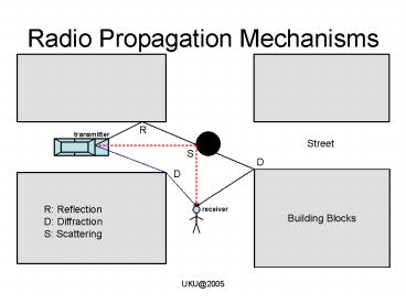
Radio Propagation Mechanisms
R
transmitter
Street
S
D
D
Building Blocks
R Reflection D Diffraction S Scattering
receiver
2
(No Transcript)
3
Long distance path loss model
- The average large-scale path loss for an
arbitrary T-R separation is expressed as a
function of distance by using a path loss
exponent n - The value of n depends on the propagation
environment for free space it is 2 when
obstructions are present it has a larger value.
Equation 11
4
Path Loss Exponent for Different Environments
5
Log-normal Shadowing
- Equation 11 does not consider the fact the
surrounding environment may be vastly different
at two locations having the same T-R separation - This leads to measurements that are different
than the predicted values obtained using the
above equation. - Measurements show that for any value d, the path
loss PL(d) in dBm at a particular location is
random and distributed normally.
6
Log-normal Shadowing- Path Loss
Then adding this random factor
Equation 12
denotes the average large-scale path loss (in dB)
at a distance d.
Xs is a zero-mean Gaussian (normal) distributed
random variable (in dB) with standard deviation
s (also in dB).
is usually computed assuming free space
propagation model between transmitter and d0 (or
by measurement).
Equation 12 takes into account the shadowing
affects due to cluttering on the propagation
path. It is used as the propagation model for
log-normal shadowing environments.
7
Log-normal Shadowing- Received Power
- The received power in log-normal shadowing
environment is given by the following formula
(derivable from Equation 12) - The antenna gains are included in PL(d).
Equation 12
8
Log-normal Shadowing, n and s
- The log-normal shadowing model indicates the
received power at a distance d is normally
distributed with a distance dependent mean and
with a standard deviation of s - In practice the values of n and s are computed
from measured data using linear regression so
that the difference between the measured data and
estimated path losses are minimized in a mean
square error sense.
9
Example of determining n and s
- Assume Pr(d0) 0dBm and d0 is 100m
- Assume the receiver power Pr is measured at
distances 100m, 500m, 1000m, and 3000m, - The table gives the measured values of received
power
10
Macrocells
- In early days, the models were based on emprical
studies - Okumura did comprehesive measurements in 1968 and
came up with a model. - Discovered that a good model for path loss was a
simple power law where the exponent n is a
function of the frequency, antenna heights, etc. - Valid for frequencies in 100MHz 1920 MHz
for distances 1km 100km
11
Okumura Model
Equation 40
- L50(d)(dB) LF(d) Amu(f,d) G(hte) G(hre)
GAREA - L50 50th percentile (i.e., median) of path loss
- LF(d) free space propagation pathloss.
- Amu(f,d) median attenuation relative to free
space - Can be obtained from Okumuras emprical plots
shown in the book (Rappaport), page 151. - G(hte) base station antenna heigh gain factor
- G(hre) mobile antenna height gain factor
- GAREA gain due to type of environment
- G(hte) 20log(hte/200) 1000m gt hte gt 30m
- G(hre) 10log(hre/3) hre lt 3m
- G(hre) 20log(hre/3) 10m gt hre gt 3m
- hte transmitter antenna height
- hre receiver antenna height
12
Hata Model
- Valid from 150MHz to 1500MHz
- A standard formula
- For urban areas the formula is
- L50(urban,d)(dB) 69.55 26.16logfc -
13.82loghte a(hre)
(44.9 6.55loghte)logd where - fc is the ferquency in MHz
- hte is effective transmitter antenna height in
meters (30-200m) - hre is effective receiver antenna height in
meters (1-10m) - d is T-R separation in km
- a(hre) is the correction factor for effective
mobile antenna height which is a function of
coverage area - a(hre) (1.1logfc 0.7)hre (1.56logfc
0.8) dB for a small to medium sized city
Equation 41
13
Microcells
- Propagation differs significantly
- Milder propagation characteristics
- Small multipath delay spread and shallow fading
imply the feasibility of higher data-rate
transmission - Mostly used in crowded urban areas
- If transmitter antenna is lower than the
surrounding building than the signals propagate
along the streets Street Microcells
14
Macrocells versus Microcells
15
Street Microcells
- Most of the signal power propagates along the
street. - The sigals may reach with LOS paths if the
receiver is along the same street with the
transmitter - The signals may reach via indirect propagation
mechanisms if the receiver turns to another
street.
16
Street Microcells
D
Building Blocks
C
B
A
Breakpoint
received power (dB)
received power (dB)
B
A
A
n2
n2
Breakpoint
1520dB
C
n4
D
n48
log (distance)
log (distance)
17
Prediction Model
Lees Prediction Model
Dalam persamaan linear,
Dalam persamaan logaritmik (dB),
Pr Daya terima pada jarak r dari
transmitter. Pro Daya terima pada jarak ro
1 mil dari transmitter. g Slope /
kemiringan Path Loss n Faktor koreksi,
digunakan apabila ada perbedaan frekuensi
antara kondisi saat eksperimen dengan kondisi
sebenarnya. ao Faktor koreksi, digunakan
apabila ada perbedaan keadaan antara kondisi
saat eksperimen dengan kondisi sebenarnya.
Kondisi saat eksperimen dilakukan, 1. Operating
Frequency 900 MHz. 2. RBS antenna 30.48 m 3.
MS antenna 3 m 4. RF Tx Power 10 watt 5. RBS
antenna Gain 6 dB over dipole l/2. 6. MS
antenna Gain 0 dB over dipole l/2.
18
Lees Prediction Model
ao faktor koreksi
Pro and g didapat dari data hasil percobaan
ao a1 . a2 . a3 . a4 . a5
in urban area (Philadelphia), Pro 10-7
mWatts g 3.68
in free space, Pro 10-4.5 mWatts g 2
in an open area, Pro 10-4.9 mWatts g
4.35
in urban area (Tokyo), Pro 10-8.4 mWatts g
3.05
in sub urban area, Pro 10-6.17 mWatts g
3.84
19
Lees Prediction Model
Correction factor to determine v in a2
n diperoleh dari percobaan / empiris
v 2, for new mobile-unit antenna heigh gt 10 m
Harga n diperoleh dari hasil percobaan
yang dilakukan oleh Okumura dan Young
v 1, for new mobile-unit antenna heigh lt 3 m
Berdasarkan eksperimen oleh Okumura n30 dB/dec
untuk Urban Area.
Berdasarkan eksperimen oleh Young n20 dB/dec
untuk Sub.Urban Area atau Open Area
n hanya berlaku untuk frekuensi operasi 30 sd.
2,000 MHz
20
Lees Prediction Model
21
Lees Pathloss Formula Untuk Berbagai Jenis
Kondisi Lingkungan
ao a1 . a2 . a3 . a4 . a5
persamaan umum,
22
Prediction Model
Okumura-Hata Prediction Model
Kelebihan mudah digunakan ( langsung
dimasukkan pada rumus jadi ) Kekurangan
tidak ada parameter eksak yang tegas antara
daerah kota, daerah suburban, maupun
daerah terbuka
- Daerah kota
Lu 69,5526,16log fC 13,83log hT a(hR)44,9
6,55 log hT log d
Dimana ,
150 ? fC ? 1500 MHz 30 ? hT ? 200 m 1 ? d ?
20 km a(hR) adalah faktor koreksi antenna mobile
yang nilainya adalah sebagai berikut
- Untuk kota kecil dan menengah,
- a(hR) (1,1 log fC 0,7 )hR (1,56 log
fC 0,8 ) dB - dimana, 1 ? hR ? 10 m
- Untuk kota besar,
- a(hR) 8,29 (log 1,54hR )2 1,1 dB
fC ? 300 MHz - a(hR) 3,2 (log 11,75hR )2 4,97 dB
fC gt 300 MHz
23
Okumura-Hata Prediction Model
- Daerah Suburban
- Daerah Open Area
24
Prediction Model
COST-231 ( PCS Extension Hata Model)
Merupakan formula pengembangan rumus Okumura Hata
untuk frekuensi PCS ( 2GHz)
dimana ,
1500 ? fC ? 2000 MHz 30 ? hT ? 200 m 1 ? d ?
20 km a(hR) adalah faktor koreksi antena mobile
yang nilainya sebagai berikut
- Untuk kota kecil dan menengah,
- a(hR) (1,1 log fC 0,7 )hR (1,56 log
fC 0,8 ) dB - dimana, 1 ? hR ? 10 m
- Untuk kota besar,
- a(hR) 8,29 (log 1,54hR )2 1,1 dB
fC ? 300 MHz - a(hR) 3,2 (log 11,75hR )2 4,97 dB
fC ? 300 MHz
25
Prediction Model
COST231 Walfish Ikegami Model
Cost231 Walfish Ikegami Model digunakan untuk
estimasi pathloss untuk lingkungan urban untuk
range frekuensi seluler 800 hingga 2000 MHz.
- Wallfisch/Ikegami model terdiri dari 3 komponen
- Free Space Loss (Lf)
- Roof to street diffraction and scatter loss
(LRTS) - Multiscreen loss (Lms)
Lf LRTS Lms
LC
Lf untuk LRTS Lms lt 0
- Lf 32.4 20 log10 R 20 log10 fc
dimana R (km) fc (MHz)
- LRTS -16.9 10 log10 W 20 log10 fc 20
log10 ?hm L?
di mana L?
-10 0.354? 0 lt ? lt 35 2.5 0.075(? - 35)
35 lt ? lt 55 4.0 0.114(? - 55) 55 lt ? lt 90
26
Prediction Model
COST231 Walfish Ikegami Model
- Lms Lbsh ka kd log10 R kf log10 fc - 9
log10 b
-18 log10 (1 ?hm ) hb lt hr ? hb gt hr
dimana Lbsh
54 hb gt hr 54 0.8hb d gt 500 m hb lt hr 54
0.8 ?hb . R 55 lt ? lt 90
ka
Catatan Lsh dan ka meningkatkan path loss
untuk hb yang lebih rendah.
18 hb gt hr 18 15 (?hb/?hr ) hb lt hr
kd
4 0.7 (fc/925 - 1 4 1.5 (fc/925 - 1)
Untuk kota ukuran sedang dan suburban dengan
kerapatan pohon cukup moderat
kf
Pusat kota metropolitan
27
Diagram Parameter
Building
Building
MOBILE
?
Building
Incident Wave
? incident angle relative to street
Building
28
(No Transcript)
29
(No Transcript)
30
(No Transcript)
31
(No Transcript)
32
(No Transcript)
33
(No Transcript)
Recommended
CrystalGraphics Presentations


