HMI, Photospheric Flows and ILCT

1
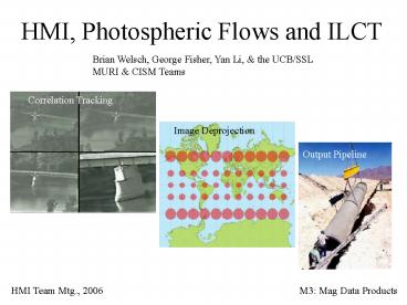
HMI, Photospheric Flows and ILCT
Brian Welsch, George Fisher, Yan Li, the
UCB/SSL MURI CISM Teams
Correlation Tracking
Image Deprojection
Output Pipeline
HMI Team Mtg., 2006
M3 Mag Data Products
2
Velocity inversions generate a 2D map
v(x1,x2)from one 2D image, f1(x1,x2), to
another, f2(x1,x2).

• The map depends upon
• the difference ?f(x1,x2) f2(x1,x2) f1(x1,x2)
• assumption(s) relating v(x1,x2) to ?f/?t, e.g.
• continuity equation, ?f/?t ?t?(vtf) 0, or
• advection equation, ?f/?t (vt??t)f 0, etc.
• Based on the assumption chosen, v(x1,x2) is not
  necessarily
• velocity e.g., group velocity of interference
  patterns.

3
Local correlation tracking (LCT) finds v(x1,x2)
by correlating subregions it assumes advection.




4) v(xi, yi) is inter- polated max. of
correlation funct
1) for ea. (xi, yi) above Bthreshold
2) apply Gaussian mask at (xi, yi)
3) truncate and cross-correlate
4
Demoulin Berger (2003) argued that LCT applied
to magnetograms does not necessarily give plasma
velocities.

• uf ? vnBh-vhBn is the flux transport velocity
• uf is the apparent velocity (2 components)
• v is the actual plasma velocity (3 comps)

Motion of flux across photosphere, uf, can be a
combination of horizontal vertical flows acting
on non-vertical fields.
5
The magnetic induction equations normal
component relates velocities to dBn/dt.

• ?Bn/?t ?h?(vnBh-vhBn) -?h?(ufBn)
• In fact, -?h?(uLCTBn) only approximates ?Bn/?t,
  so
• uLCT ? uf
• Inductive LCT (ILCT) finds uf that matches ?Bn/?t
  exactly and closely matches uLCT.
• Writing ufBn -?h? ?h x(? n), we find
• ? via ?Bn/?t ?h2?
• ? by assuming uf uLCT, so ?h2? - ?h x(
  uLCTBn)

6
Aside fundamentally, two components of uf(x1,x2)
cannot determine three components of plasma
velocity, v(x1,x2).

• Hence, other velocity fields v(x1,x2) consistent
  with ?Bn/?t can be found.
• Other techniques available include
• Minimum Energy Fit (MEF, Longcope, 2004)
• Differential LCT (DLCT) Differential Affine
  Velocity Estimator (DAVE) (Schuck, 2006)

7
The FLCT codes current version combines pro-
grams written in IDL C, and open source code.

• IDL
• C
• Standard C library routines stdio.h, stdlib.h,
  math.h
• Fastest Fourier Transform in the West (FFTW), v.
  3.0
• The executable has been compiled tested on
  several architectures.
• Linux
• Solaris
• Windows
• Macintosh

8
Matching HMIs 10-minute vector magnetogram
cadence will be challenging.

• HMI has Npix 107 pixels within 60o of disk
  center.
• - MDIs 10242 ? HMIs 40962 ?
  x 16
• - MDI, w/in 30o ? HMI, w/in 60o ? x
  2.5
• We track pixels with Bn gt Bthresh 20G
• 25 of Npix at solar max.
• 5 of Npix at solar min.
• FLCT speed is linear in Npix correlated.
• - ?t (1 sec/100 pix) x (2.5 x 106 pix) 2.5 x
  104 sec 7 hr!
• - at solar min., w/ Bthresh 100G (1 of
  Npix), ?t 20 min.

9
Velocity estimates work from difference images,
so temporal artifacts must be removed.

• IVM difference images of BLOS in AR 9026, with a
  4 min. cadence, show large-scale, alternating
  field fluctuations that inhibit accurate tracking.

10
Accurate velocity estimates also require
deprojection of full-disk magnetograms.

• Away from disk center, flows with a component
  along LOS are foreshortened by curvature of the
  solar surface.
• Conformal deprojections, e.g., Mercator, locally
  preserve angles scales are distorted, but easily
  fixed.
• This is optimal for tracking, since neither flow
  component is biased by the deprojection.
• (Apparent changes in lengths perpendicular to the
  LOS from center-to-limb are negligible.)

11
FLCT was initially tested using a known image.
We found FLCT could accurately reconstruct the
imposed flow.
12
FLCT was also tested on magnetograms with imposed
differential rotation again, recovering the
input flow.
White dots are imposed differential rotation
profile red dots are raw velocities from
Mercator projection green are properly rescaled
white diamonds are latitudinally binned averages
of green dots.
13
We have implemented a preliminary, automated
Magnetic Evolution Pipeline (MEP).

• http//solarmuri.ssl.berkeley.edu/welsch/public/d
  ata/Pipeline/
• cron checks for new magnetograms with wget
• New magnetograms are downloaded, deprojected, and
  tracked using FLCT.
• The output stream includes deprojected m-grams,
  FLCT flows (.png graphics files ASCII data
  files), and tracking parameters.
• Full documentation all codes are on line.

14
Several performance-enhancing modifications to
FLCT were implemented and more are planned.

• Sub-pixel interpolation was made more efficient.
• Correlation is now accomplished by spawning a C
  subroutine that employs FFTW.
• FLCT is readily parallelizable we envision this
  soon.
• Computing velocities in neighborhoods, as opposed
  to each pixel, is another way to increase speed.

15
Conclusions

• Accurate flow estimates will require
• deprojection of full-disk magnetograms, and
• careful temporal filtering.
• Matching planned data cadences will be
  challenging. Solutions
• parallelization
• find v(x1,x2) on tiles, not every pixel
• more restricitve Bn thresholding
• Essential tools for an LCT pipeline are in place.

16
References

• Démoulin Berger, 2003 Magnetic Energy and
  Helicity Fluxes at the Photospheric Level,
  Démoulin, P., and Berger, M. A. Sol. Phys., v.
  215, 2, p. 203-215.
• Longcope, 2004 Inferring a Photospheric Velocity
  Field from a Sequence of Vector Magnetograms The
  Minimum Energy Fit, ApJ, v. 612, 2, p.
  1181-1192.
• Schuck, 2005 Tracking Magnetic Footpoints with
  the Magnetic Induction Equation, ApJ (submitted,
  2006)
• Welsch et al., 2004 ILCT Recovering
  Photospheric Velocities from Magnetograms by
  Combining the Induction Equation with Local
  Correlation Tracking, Welsch, B. T.,
  Fisher, G. H., Abbett, W.P., and Regnier, S.,
  ApJ, v. 610, 2, p. 1148-1156.

17
Yangs e-mail.

• It would be great if you can talk about your
  ILCT method/ code
• during the session. Because this session is data
  products session,
• briefly summarize your algorithm first, and
  then focus on
• addressing following issues
• Nature of the codes (Language, etc)
• Additional supporting software (IDL, MATHLIB,
  ...)
• Computational requirements (run time estimate,
  system requirements, etc)
• Requirements for the input data format of the
  output products
• Potential challenges, test procedures, target
  date for completion of codes, etc...
• Time is 15 minutes, but leave 5 minutes for
  further discussion.