
Exact Inference Last Class - PowerPoint PPT Presentation
1 / 21
Title:
Exact Inference Last Class
Description:
Imagine Markov chain in which each state is an assignment of values to each variables. ... The idea of the burn in period is to stabilize chain ... – PowerPoint PPT presentation
Number of Views:57
Avg rating:3.0/5.0
Title: Exact Inference Last Class
1
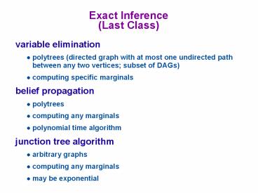
Exact Inference(Last Class)
- variable elimination
- polytrees (directed graph with at most one
undirected path between any two vertices subset
of DAGs) - computing specific marginals
- belief propagation
- polytrees
- computing any marginals
- polynomial time algorithm
- junction tree algorithm
- arbitrary graphs
- computing any marginals
- may be exponential
2
Computational Complexity of Exact Inference
- Exponential in number of nodes in a clique
- need to integrate over all nodes
- Goal is to find a triangulation that yields the
smallest maximal clique - NP-hard problem
- ?Approximate inference
3
Approximate Inference
- Exact inference algorithms exploit conditional
independencies in joint probability distribution. - Approximate inference exploits the law of large
numbers. - sums and products of many terms behave in simple
ways - Approximate inference involves sampling.
- Appropriate algorithm depends on
- can we sample from p(x)?
- can we evaluate p(x)?
- can we evaluate p(x) up to the normalization
constant?
4
Monte Carlo
- Instead of obtaining p(x) analytically, sample.
- draw i.i.d. samples x(i), i 1 ... N
- e.g., 20 coin flips with 11 heads
- With enough samples, you can estimate even
continuous distributions empirically. - Easy case
- you can sample from p(x) directly
- e.g., Bernoulli, Gaussian random variables
- Hard cases
- can evaluate p(x)
- can evaluate p(x) up to proportionality constant
5
Rejection Sampling
- Cannot sample from p(x), but can evaluate p(x) up
to proportionality constant. - Instead of sampling from p(x), use an
easy-to-sample proposal distribution q(x). - p(x) lt M q(x), M lt 8
- Reject proposals with probability p(x)/Mq(x)
6
Importance Sampling
- Uses an easily sampled proposal distribution q(x)
- Assuming p(x) can be evaluated, reweight each
sample by w p(x(i))/q(x(i)) - Find q that selects important cases
- important cases have most impact on estimate,
i.e., large weight - ? efficiency (fewer samples required)
X
t
7
Importance Sampling
- When normalizing constant of p(x) is unknown,
it's still possible to do importance sampling
with w(i) - w(i) p(x(i)) / q(x(i))
- w(i) w(i) / ?j w(j)
- Note that any scaling constant in p(.) will be
removed by the normalization.
8
MCMC
- Imagine Markov chain in which each state is an
assignment of values to each variables. - x1 ? x2 ? x3 ? ...
- Procedure
- Start x in a random state
- Repeatedly sample over many time steps (can
condition on some elements of x) - After sufficient burn in, x reaches a stationary
distribution. - Use next s samples to form empirical
distribution - Idea construct chain to spend more time in the
most important regions.
9
Example Boltzmann Machine
- http//www.cs.cf.ac.uk/Dave/JAVA/boltzman/Necker.h
tml
10
Burn In
- The idea of the burn in period is to stabilize
chain - i.e., end up at a point that doesn't depend on
where you started - e.g., person's location as a function of time
- Justifies arbitrary starting point.
- Mixing time
- how long it takes to move from initial
distribution to p(x) - Transition matrix must obey two properties
- 1. Irreducibility (can get from any state to any
other) - 2. Aperiodicity (cannot get trapped in cycles)
- MCMC Sampler transition matrix that has the
target distribution, p(x) as its asymptotic
distribution
11
Choice of Proposal Distribution Matters
- E.g., continuous distribution, one variable,
Gaussian proposal distribution, varying std
deviation
12
Gibbs Sampling
- A version of MCMC in which
- at each step, one variable xi is selected (random
or fixed seq.) - conditional distribution is estimated p(xi
xU\i) - a value is sampled from this distribution
- the sample replaces the previous value of xi
- Assumes efficient sampling of cond. distribution
- Efficient if Ci is small includes cliques for
parents, children, and children's parents
a.k.a. Markov blanket - Normalization term is often the tricky part
cliques containing xi
13
Gibbs Sampling(Andrieu notation)
- Proposal distribution
- Algorithm
14
Metropolis Algorithm
- Does not require computation of conditional
probabilities (and hence normalization) - Procedure
- at each step, one variable xi is selected (at
random or according to fixed sequence) - choose a new value for variable from proposal
distribution q - accept new value with probability
proposed value
15
Metropolis Algorithm(Andrieu notation)
- Proposal distribution is symmetric.
- i.e., q(xx) q(xx)
- e.g., mean zero Gaussian
- In the general case, a.k.a. Metropolis-Hastings
Intuition - q ratio tests how easy is it to get back to where
you came from - ratio is 1 for Metropolis algorithm
16
(No Transcript)
17
Particle Filters
- Time-varying probability density estimation
- E.g., tracking individual from GPS coordinates
- state (actual location) varies over time
- GPS reading is a noisy indication of state
- Could be used for HMM-like models that have no
easy inference procedure - Basic idea
- represent density at time t by a set of samples
(a.k.a. particles) - weight the samples by importance
- perform sequential Monte Carlo update,
emphasizing the important samples
18
(No Transcript)
19
Variational Methods
- Like importance sampling, but...
- instead of choosing a q(.) in advance, consider a
family of distributions qv(.) - use optimization to choose a particular member of
this family - optimization finds a qv(.) that is similar to the
true distribution p(.) - Optimization
- minimize variational free energy
Kullback-Leibler divergencebetween p and q
20
Variational MethodsMean Field Approximation
- Restrict q to the family of factorized
distributions - Procedure
- initialize approximate marginals q(xi) for all i
- pick a node at random
- update its approximate marginal fixing all others
- sample from q and to obtain an x(t) and use
importance sampling estimate
21
Variational MethodsBethe Free Energy
- Approximate marginals at both single nodes as
well as on cliques - Yields a better approximation of free energy-gt
yields a better estimate of p - Do a lot of fancy math and what do you get?
- loopy belief propagation
- i.e., same message passing algorithm as for
tree-based graphical models - Appears to work very well in practice
Recommended
CrystalGraphics Presentations


