
Tanks in series model - PowerPoint PPT Presentation
1 / 30
Title:
Tanks in series model
Description:
Tanks in series model. We have already seen that multiple MFRs in series approach ... quantitative analysis of the non-ideality as characterized by E curves (Fig.14.1) ... – PowerPoint PPT presentation
Number of Views:906
Avg rating:3.0/5.0
Title: Tanks in series model
1
Tanks in series model
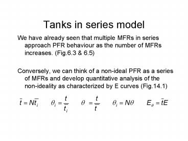
- We have already seen that multiple MFRs in series
approach PFR behaviour as the number of MFRs
increases. (Fig.6.3 6.5) - Conversely, we can think of a non-ideal PFR as a
series of MFRs and develop quantitative analysis
of the non-ideality as characterized by E curves
(Fig.14.1)
2
Fig. 6.3
3
Fig. 6.5
4
Fig. 14.1
5
Tracer balance on first tank
- Recall, generally for MFR
- input output accumulation (no reaction
term for tracer) - Assuming instantaneous addition of tracer pulse,
no more input after time 0.
6
Tracer balance on subsequent tanks
- input output accumulation (no reaction
term for tracer) - The second tank receives time varying input from
tank 1 - The third tank receives time varying input from
tank 2 - etc.
- The solutions to this set of equations are
summarized in Box 3 and Fig.14.2
7
Box 3
8
Figure 14.2
9
Observations on Fig.14.2
- The E? curve for the entire assembly (left
figure) starts resembling a PFR E? curve as N
increases. - I.e overall spread decreases.
- The E? curves for the individual reactors (right
figure, E?i) get flatter (spread increases) as
we move away from the feed end. - Note however, that the spread for the individual
tanks are measured relative to the individual
mean residence times whereas the spread for the
system as a whole is measured relative to the
system mean residence time.
10
RTD for the tanks in series model (Fig.14.3)
- The spread or flatness of a distribution can be
quantified by the variance - Fig 14.3 shows the relation between N and ?2, as
well as E?
Where ? is the mean and n is the number of
observations
11
Fig.14.3
12
One-shot tracer input
- In tracer studies, the input does not have to be
an instantaneous spike. The input can be
characterized by ??in2 - And the output by ??out2 (Fig. 14.4)
- The tanks in series model then says
- Where ?t is the time difference between the two
peaks
13
(No Transcript)
14
Example 14.2 (Fig. E14.2)
- Estimating the location of a spill in a river
from the difference of spread at two downstream
observation points. - Over 119 miles ?the spread increases from 10.5 hr
to 14 hr - By considering ?that ?2 is proportional to
distance we can deduce that an instantaneous
spill (pulse input) could have occurred 272
miles upstream, or, a sloppy input could have
occurred closer.
15
(Fig. E14.2)
16
(No Transcript)
17
miles
18
(No Transcript)
19
- Using the fact that the peak at Cincinnati
occurred 26 hours after the peak at Portsmouth,
and the ??2 expression for the tanks-in-series
model, we can find, for this stretch of river
20
Example 14.3 (Fig. E14.3a)
- From compartment models we know that multiple
decaying peaks is a sign of recirculation
(Fig.12.1, p.285) - Analyzing Fig E14.3a, we arrive at a tanks in
series model depicted in Fig. E14.3b, 14.3c,
14.3d.
21
(No Transcript)
22
Fig E14.3a
23
(No Transcript)
24
(No Transcript)
25
Fig. E14.3b, 14.3c, 14.3d
26
Example 14.4 (Fig E14.4a and 14.4b)
- Vessel E curve from ??in2 and ??out2
- Equations used for tanks in series model
27
(No Transcript)
28
(Fig E14.4a and 14.4b)
29
(No Transcript)
30
(No Transcript)
Recommended
CrystalGraphics Presentations


