Multiple Regression

1
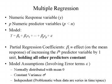
Multiple Regression

• Numeric Response variable (y)
• p Numeric predictor variables (p lt n)
• Model
• Y b0 b1x1 ??? bpxp e
• Partial Regression Coefficients bi ? effect (on
  the mean response) of increasing the ith
  predictor variable by 1 unit, holding all other
  predictors constant
• Model Assumptions (Involving Error terms e )
• Normally distributed with mean 0
• Constant Variance s2
• Independent (Problematic when data are series in
  time/space)

2
Example - Effect of Birth weight on Body Size in
Early Adolescence

• Response Height at Early adolescence (n 250
  cases)
• Predictors (p6 explanatory variables)
• Adolescent Age (x1, in years -- 11-14)
• Tanner stage (x2, units not given)
• Gender (x31 if male, 0 if female)
• Gestational age (x4, in weeks at birth)
• Birth length (x5, units not given)
• Birthweight Group (x61,...,6 lt1500g (1),
  1500-1999g(2), 2000-2499g(3), 2500-2999g(4),
  3000-3499g(5), gt3500g(6))

Source Falkner, et al (2004)
3
Least Squares Estimation

• Population Model for mean response

• Least Squares Fitted (predicted) equation,
  minimizing SSE

• All statistical software packages/spreadsheets
  can compute least squares estimates and their
  standard errors

4
Analysis of Variance

• Direct extension to ANOVA based on simple linear
  regression
• Only adjustments are to degrees of freedom
• DFR p DFE n-p (pp1Parameters
  )

5
Testing for the Overall Model - F-test

• Tests whether any of the explanatory variables
  are associated with the response
• H0 b1???bp0 (None of the xs associated with
  y)
• HA Not all bi 0

6
Example - Effect of Birth weight on Body Size in
Early Adolescence

• Authors did not print ANOVA, but did provide
  following
• n250 p6 R20.26
• H0 b1???b60 HA Not all bi 0

7
Testing Individual Partial Coefficients - t-tests

• Wish to determine whether the response is
  associated with a single explanatory variable,
  after controlling for the others
• H0 bi 0 HA bi ? 0 (2-sided
  alternative)

8
Example - Effect of Birth weight on Body Size in
Early Adolescence
Controlling for all other predictors, adolescent
age, Tanner stage, and Birth length are
associated with adolescent height measurement
9
Comparing Regression Models

• Conflicting Goals Explaining variation in Y
  while keeping model as simple as possible
  (parsimony)
• We can test whether a subset of p-g predictors
  (including possibly cross-product terms) can be
  dropped from a model that contains the remaining
  g predictors. H0 bg1bp 0
• Complete Model Contains all p predictors
• Reduced Model Eliminates the predictors from H0
• Fit both models, obtaining sums of squares for
  each (or R2 from each)
• Complete SSRc , SSEc (Rc2)
• Reduced SSRr , SSEr (Rr2)

10
Comparing Regression Models

• H0 bg1bp 0 (After removing the effects of
  X1,,Xg, none of other predictors are associated
  with Y)
• Ha H0 is false

P-value based on F-distribution with p-g and n-p
d.f.
11
Models with Dummy Variables

• Some models have both numeric and categorical
  explanatory variables (Recall gender in example)
• If a categorical variable has m levels, need to
  create m-1 dummy variables that take on the
  values 1 if the level of interest is present, 0
  otherwise.
• The baseline level of the categorical variable is
  the one for which all m-1 dummy variables are set
  to 0
• The regression coefficient corresponding to a
  dummy variable is the difference between the mean
  for that level and the mean for baseline group,
  controlling for all numeric predictors

12
Example - Deep Cervical Infections

• Subjects - Patients with deep neck infections
• Response (Y) - Length of Stay in hospital
• Predictors (One numeric, 11 Dichotomous)
• Age (x1)
• Gender (x21 if female, 0 if male)
• Fever (x31 if Body Temp gt 38C, 0 if not)
• Neck swelling (x41 if Present, 0 if absent)
• Neck Pain (x51 if Present, 0 if absent)
• Trismus (x61 if Present, 0 if absent)
• Underlying Disease (x71 if Present, 0 if absent)
• Respiration Difficulty (x81 if Present, 0 if
  absent)
• Complication (x91 if Present, 0 if absent)
• WBC gt 15000/mm3 (x101 if Present, 0 if absent)
• CRP gt 100mg/ml (x111 if Present, 0 if absent)

Source Wang, et al (2003)
13
Example - Weather and Spinal Patients

• Subjects - Visitors to National Spinal Network in
  23 cities Completing SF-36 Form
• Response - Physical Function subscale (1 of 10
  reported)
• Predictors
• Patients age (x1)
• Gender (x21 if female, 0 if male)
• High temperature on day of visit (x3)
• Low temperature on day of visit (x4)
• Dew point (x5)
• Wet bulb (x6)
• Total precipitation (x7)
• Barometric Pressure (x7)
• Length of sunlight (x8)
• Moon Phase (new, wax crescent, 1st Qtr, wax
  gibbous, full moon, wan gibbous, last Qtr, wan
  crescent, presumably had 8-17 dummy variables)

Source Glaser, et al (2004)
14
Modeling Interactions

• Statistical Interaction When the effect of one
  predictor (on the response) depends on the level
  of other predictors.
• Can be modeled (and thus tested) with
  cross-product terms (case of 2 predictors)
• E(Y) a b1X1 b2X2 b3X1X2
• X20 ? E(Y) a b1X1
• X210 ? E(Y) a b1X1 10b2 10b3X1
• (a 10b2)
  (b1 10b3)X1
• The effect of increasing X1 by 1 on E(Y) depends
  on level of X2, unless b30 (t-test)

15
Regression Model Building

• Setting Possibly a large set of predictor
  variables (including interactions).
• Goal Fit a parsimonious model that explains
  variation in Y with a small set of predictors
• Automated Procedures and all possible
  regressions
• Backward Elimination (Top down approach)
• Forward Selection (Bottom up approach)
• Stepwise Regression (Combines Forward/Backward)
• Cp Statistic - Summarizes each possible model,
  where best model can be selected based on
  statistic

16
Backward Elimination

• Select a significance level to stay in the model
  (e.g. SLS0.20, generally .05 is too low, causing
  too many variables to be removed)
• Fit the full model with all possible predictors
• Consider the predictor with lowest t-statistic
  (highest P-value).
• If P gt SLS, remove the predictor and fit model
  without this variable (must re-fit model here
  because partial regression coefficients change)
• If P ? SLS, stop and keep current model
• Continue until all predictors have P-values below
  SLS

17
Forward Selection

• Choose a significance level to enter the model
  (e.g. SLE0.20, generally .05 is too low, causing
  too few variables to be entered)
• Fit all simple regression models.
• Consider the predictor with the highest
  t-statistic (lowest P-value)
• If P?? SLE, keep this variable and fit all two
  variable models that include this predictor
• If P gt SLE, stop and keep previous model
• Continue until no new predictors have P?? SLE

18
Stepwise Regression

• Select SLS and SLE (SLEltSLS)
• Starts like Forward Selection (Bottom up process)
• New variables must have P ? SLE to enter
• Re-tests all old variables that have already
  been entered, must have P ? SLS to stay in model
• Continues until no new variables can be entered
  and no old variables need to be removed

19
All Possible Regressions - Cp

• Fits every possible model. If K potential
  predictor variables, there are 2K-1 models.
• Label the Mean Square Error for the model
  containing all K predictors as MSEK
• For each model, compute SSE and Cp where p is
  the number of parameters (including intercept) in
  model

• Select the model with the fewest predictors that
  has Cp ? p or less

20
Regression Diagnostics

• Model Assumptions
• Regression function correctly specified (e.g.
  linear)
• Conditional distribution of Y is normal
  distribution
• Conditional distribution of Y has constant
  standard deviation
• Observations on Y are statistically independent
• Residual plots can be used to check the
  assumptions
• Histogram (stem-and-leaf plot) should be
  mound-shaped (normal)
• Plot of Residuals versus each predictor should be
  random cloud
• U-shaped (or inverted U) ? Nonlinear relation
• Funnel shaped ? Non-constant Variance
• Plot of Residuals versus Time order (Time series
  data) should be random cloud. If pattern appears,
  not independent.

21
Detecting Influential Observations

• Studentized Residuals Residuals divided by
  their estimated standard errors (like
  t-statistics). Observations with values larger
  than 3 in absolute value are considered outliers.
• Leverage Values (Hat Diag) Measure of how far
  an observation is from the others in terms of the
  levels of the independent variables (not the
  dependent variable). Observations with values
  larger than 2p/n are considered to be
  potentially highly influential, where p is the
  number of predictors and n is the sample size.
• DFFITS Measure of how much an observation has
  effected its fitted value from the regression
  model. Values larger than 2sqrt(p/n) in absolute
  value are considered highly influential. Use
  standardized DFFITS in SPSS.

22
Detecting Influential Observations

• DFBETAS Measure of how much an observation has
  effected the estimate of a regression coefficient
  (there is one DFBETA for each regression
  coefficient, including the intercept). Values
  larger than 2/sqrt(n) in absolute value are
  considered highly influential.
• Cooks D Measure of aggregate impact of each
  observation on the group of regression
  coefficients, as well as the group of fitted
  values. Values larger than 4/n are considered
  highly influential.
• COVRATIO Measure of the impact of each
  observation on the variances (and standard
  errors) of the regression coefficients and their
  covariances. Values outside the interval 1 /-
  3p/n are considered highly influential.

23
Variance Inflation Factors

• Variance Inflation Factor (VIF) Measure of how
  highly correlated each independent variable is
  with the other predictors in the model. Used to
  identify Multicollinearity.
• Values larger than 10 for a predictor imply large
  inflation of standard errors of regression
  coefficients due to this variable being in model.
• Inflated standard errors lead to small
  t-statistics for partial regression coefficients
  and wider confidence intervals

24
Nonlinearity Polynomial Regression

• When relation between Y and X is not linear,
  polynomial models can be fit that approximate the
  relationship within a particular range of X
• General form of model

• Second order model (most widely used case,
  allows one bend)

• Must be very careful not to extrapolate beyond
  observed X levels