Ch 11 Return and Risk: The Capital Asset Pricing Model CAPM

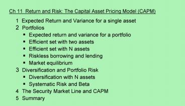
1
Ch 11 Return and Risk The Capital Asset Pricing
Model (CAPM)

• 1 Expected Return and Variance for a single
  asset
• Portfolios
• Expected return and variance for a portfolio
• Efficient set with two assets
• Efficient set with N assets
• Riskless borrowing and lending
• Market equilibrium
• Diversification and Portfolio Risk
• Diversification with N assets
• Systematic Risk and Beta
• 4 The Security Market Line and CAPM
• 5 Summary

2
Main Idea

• What is an appropriate measure of risk?
• If you hold single asset, standard deviation of
  the asset is a good measure of the risk.
• If you hold a widely diversified portfolio, the
  beta of the asset is a good measure of the risk
  of the asset.
• Average return of the asset is a good measure of
  the expected return in both cases.

3
1. Expected Return and Variance

• Goal To derive a relation between return and
  risk in the form of
• E(Ri) Rf ?i E(Rm) Rf  
• where
• Rf ? risk free rate (e.g., T-bill rate)
• Rm ? return on market portfolio
• (e.g., a value-weighted portfolio of all
  TSE stocks)
• ?i Measure of risk of asset i
• ? Cov (asseti, market portfolio) / Var
  (market portfolio)
• In order to measure and develop models for the
  relation between risk and return, we need some
  formal statistical measures.

4
1.1 Calculating the Expected Return

• Example 1 Average of two scores 80 and 60
  (8060)/2 70.
• Example 2 You feel youd get 80 and 60 in a
  finance course with equal probability of 0.5 and
  0.5. What do you expect to get?

• In Example 1, it is as if equal probabilities
  are assigned to calculate the mean mean
  (0.580) (0.560) (8060)/2 70.
• We can generalize mean sum of (probpossible
  outcome), i.e.,
• E(x) sum (Pi
  xi) ? ?I (Pi xi)

5
Example Calculating the Expected Return

• Example 3 You feel youd get 80 and 60 in a
  finance course with probability of 0.4 and 0.6.
  What do you expect to get?
• Qu What are E(x2), E(x3 - 3x), or in general,
  E anything ?
• E(x2) sum (Pi xi2)
• E(x3 - 3x) sum ( Pi (xi3 - 3xi) )
• E (anything) sum (Pi possible outcome i of
  anything), i.e.,
• E f(x) sum Pi f(xi) ? ?I Pi f(xi)
  

6
1.2 Calculating variance

• Example 1 You expect to get 80 and 60 in a
  finance course with probability of 0.4 and 0.6.
  What is variance of your score?
• variance(x) ? sx2 ? E (x - E(x))2 . Why
  squared?
• Recall E anything sum (Pi possible outcome
  i of anything).
• sx2 ? E (x - E(x) )2 sum Pi possible
  outcome of (xi - E(x))2

7
1.2 Calculating variance

• Why standard deviation?
• Variance isn't in the same units as the
  mean--it's in (unit)2. It is often useful to
  work with standard deviation which is in the
  units as the mean.
• 1.3 Calculating covariance and correlation
• A measure of how random variables move together
  is covariance.
• If we have two random variables, X and Y, their
  covariance is defined as cov (x, y) ? E (x -
  E(x)) (y - E(y))

8
1.3 Calculating covariance and correlation

• Example 1 You feel youd get 80 and 60 in a
  finance and 70 and 90 in an accounting course
  with probability of 0.4 and 0.6. Find out the
  mean, variance and standard deviation of finance
  (x) and accounting (y) scores.
• E(x) 68 sx2 96 sx 9.8
• E(y) 82 sy2 96 sy 9.8
• What is the covariance of your finance and
  accounting scores?
• Recall E anything sum (Pi possible outcome
  i of anything).
• cov (x, y) ? E (x - E(x)) (y - E(y))
• sum Pi possible outcome of
  (xi - E(x)) (yi - E(y))
• ?I Pi (xi - E(x)) (yi -
  E(y))

9
1.2 Calculating covariance and correlation

• cov (x, y) ?I Pi (xi - E(x)) (yi - E(y))

corr (x, y) cov (x, y) / (sxsy) . Why using
correlation? corr (x, y) always lies between -1
and 1. corr (x, y) 1 perfectly positive
correlation corr (x, y) -1 perfectly
negative correlation corr (x, y) 0
independent
10
Qu 12.7 Calculation of mean, variance covariance
Using the following returns, calculate the
average returns, the variances, the standard
deviations, covariance and correlation for stocks
X and Y.
When you use actual data (i.e., no probabilities)
and calculate moments, follow these rules 1.
E(X) sum all xi and divide by T (no of
observations) 2. var E (X - E(X))2 sum
all (xi - E(X))2 divide by (T-1) 3. cov E
(X-E(X))(Y-E(Y)) sum all
(xi-E(X))(yi-E(Y)) and divide by (T-1)
11
Qu Calculation of mean, variance covariance
12
Qu. Calculation of mean, variance covariance
with Probability distribution
13
Evidence on Covariance and Correlation

• (1) Stock returns are serially uncorrelated.
• If stock returns are high one year then, you
  can't use this information to predict whether
  returns in the subsequent year will be high or
  low. This evidence is important to market
  efficiency.
• (2) Most stocks are positively correlated to the
  market portfolio important evidence for our
  discussion of asset pricing model.
• market portfolio a value-weighted portfolio of
  all the stocks in the economy (or as a proxy, all
  stocks on the NYSE or TSE).

14
Statistical Review Conclusion

• The main thing is to have an intuitive
  understanding of what these statistics mean.
• Arithmetic mean is a measure of how much you
  can expect to receive if you hold a stock for a
  year.
• The variance and standard deviation are
  measures of how variable the returns are likely
  to be. The higher the variance or standard
  deviation the greater the variation.
• Covariance and correlation are measures of
  whether two variables move together or in
  opposite directions.
• Move together positive
• Move in opposite directions negative
  
• Independent zero.

15
2. Diversification

• 2.1 Mean and variance of portfolio
• Suppose we have 1,000 to invest, and there are
  two risky assets  
•  
• We could invest it all in asset 1 or all in asset
  2. However, we may do better off by taking a
  combination of asset 1 and asset 2, i.e.,
  diversification may provide better result than by
  taking 1 or 2 alone. Let us see
• Suppose correlation between asset 1 and 2s
  return is 0.5. Let x1 be the proportion of our
  wealth invested in asset 1. (What is proportion
  of wealth invested asset 2?)

16
2.1 Mean and variance of a portfolio

• Mean return and variance of a portfolio with two
  assets
• When x10, we invest entire wealth in asset 2.
  The portfolio has a mean return of 8 and ? of
  0.05.
• When x11, we invest entire wealth in asset 1.
  The portfolio has a mean return of 5 and ? of
  0.03.
•  

17
2.1 Mean and variance of a portfolio

• What will happen in-between?
• E(Rp) x1 E(R1) (1 - x1) E(R2) (1)
• ?p2 x12 ?12 (1 - x1)2 ?22 2x1(1 - x1) cov
  (R1, R2) (2)
• Note Recall ?12 ? Corr (R1, R2) cov (R1,
  R2)/(?1 ?2).
• Sometimes, we use ?12 ?1 ?2 instead of cov (R1,
  R2).
• Suppose that x10.1. We can calculate the mean
  return and ? of the portfolio using equations (1)
  and (2). We can do the same calculation for
  x10.2, 0.3,.,x11, and fill up the following
  table.
• Using these results, we can draw the following
  chart

18
2.1 Mean and variance of a portfolio
19
2.1 Mean and variance of a portfolio
20
2.2 Relation between ? and investment
opportunity set

• Figure 1 shows investment opportunity set,
  i.e., mean and standard deviations for all
  possible combinations of assets 1 and 2.
• For Figure 1, we assume corr 0.5. Let ?
  denote correlation. Correlation lies between -1
  and 1. How investment does investment
  opportunity set change when ? changes?

21
2.2 Relation between ? and investment
opportunity set
Result The lower the ?, the greater the benefit
from diversification.
22
2.3 Efficient frontier with N assets
C
B minimum variance portfolio
mean
ABC minimum variance frontier
B
BC efficient frontier
Shaded area investment opportunity set
A
standard deviation
Diversification with N assets covariance among
assets affects the variance of a portfolio with N
assets. We will look at this issue at section
3.1.
23
2.4 Riskless Borrowing and Lending

• With a risk-free asset available and the
  efficient frontier identified, an investor
  chooses the capital allocation line with the
  steepest slope.

CML
return
efficient frontier
rf
?P
24

• Note that the risk-return relation of a porfolio
  of risk free asset and a risky asset Q is
  represented by a straight line between the risk
  free rate on y-axis and the risk asset Q.
• (proof optional material)

25
2.4 Riskless Borrowing and Lending

• With the capital allocation line identified, an
  investor chooses a point along the linesome
  combination of the risk-free asset and a risky
  portfolio M.

• CML capital markets line

CML
return
efficient frontier
M
rf
?P
26
The Separation Property

• The Separation Property states that investors can
  separate their risk aversion from their choice of
  the risky portfolio.
• Implications portfolio choice can be separated
  into two tasks (1) determine the optimal risky
  portfolio, and (2) selecting a point on the CML.

CML
return
efficient frontier
M
rf
?P
27
Market equilibrium

• In a world with homogeneous expectations, the
  portfolio of risky asset is the same for all
  investors.
• In capital market equilibrium, demand equal
  supply.
• The portfolio of risky asset in equilibrium is
  called the market portfolio.
• market portfolio A portfolio of all stocks in
  the market. Portfolio weight of stock i is
  equal to the proportion of stock is market value
  to the market value of all stocks in the market
  portfolio.  
• If total value of stock 1 is 10 billion and the
  total value of the market portfolio is 1,000
  billion. Then x110/1,0001. We denote the
  market portfolio by M.

28
3. Diversification and portfolio risk

• We know how investors behave in a world with risk
  free asset, and with homogeneous expectations.
• Investors will hold the same risky portfolio M,
  and risk free asset in their portfolio. The
  proportions of the risky and risk free assets are
  dependent on the investors risk aversion.
• The risky portfolio M is the market portfolio.
• Next Qu what is the risk-return relation among
  assets in portfolio M?

29
3. Diversification and portfolio risk
3.1. diversification with N assets Qu how much
risk can we eliminate by diversification?
30
3.1 diversification

• diversification diversification eliminates
  some, but not all of the risk.
• Systematic risk risk that influences overall
  stock market, such as GNP, or interest rate. It
  can't be diversified away
• Unsystematic risk risk that influences
  single industries, or individual firms such RD
  results or a change in CEO.
• A stock thus has two components of risk
  systematic and unsystematic risk. One can
  eliminate most of unsystematic risk with about
  15-30 stocks.

31
3.2 A principle

• A principle The reward for bearing risk
  depends only on the systematic risk of an
  investment.
• The market does not reward bearing unsystematic
  risk, since these risk can be diversified away in
  a reasonably large portfolio.
• Hence it is systematic risk which is
  important. Suppose stock A and B have the same
  expected return. A has a higher variance, but
  lower systematic risk than stock B. The stock A
  may be much more desirable than stock B with a
  lower variance.

32
3.3 Systematic risk and beta (ß)

• So, it is systematic risk, not the total risk
  of a stock, which is important. We can say that
  a stock has a high risk if it has large
  systematic risk. But how do we know that a stock
  has large systematic risk? I.E., how do we
  measure systematic risk of a stock?
• Answer Beta (ß),
• where ?i ? Cov (Ri, Rm) / Var (Rm), and Rm is
  return on the market portfolio.

33
3.3 Systematic risk and beta (ß)

• Basic intuition about ß
• ß measures how much systematic risk a stock has
  relative to the market portfolio (or an average
  asset). By definition, ß of the market portfolio
  is 1.
• Recall that systematic risk influences
  overall stock market. If a stocks return
  co-moves a lot with overall stock market, this
  stock has high systematic risk. That is why you
  see Cov (Ri, Rm) in numerator of definition of ß.

34

• Interpretation of ß
• (1) It is reasonable to say that the market
  portfolio has (almost) systematic risk only,
  since diversification eliminates (nearly) all of
  unsystematic risk.
• Consider the extent to which the variance of the
  market portfolio change if we change the amount
  of the stock in the portfolio.
• That is ß, i.e., the contribution of the stock to
  the variance of the market portfolio (or in
  mathematical term (? ?m2 / ?xi)).

35

• ß measures sensitivity of a stocks return to
  movements in overall market. By definition, ßm
  Cov (Rm, Rm) / Var (Rm) 1. That is, ß of
  market portfolio is 1.
• Thus stocks with a ß gt 1 tend to be sensitive to
  movements in the market--they magnify these
  movements. Stocks with a ß lt 1 are relatively
  insensitive to movements in the market.

36
3.3 Systematic risk and beta (ß)..

• High ß stock Low ß stock
• ß regression coefficient

37
3.3 Systematic risk and beta (ß)..
Beta Coefficients for Selected Companies
Canadian Co. Beta Bank of Nova
Scotia 0.65 Bombardier 0.71 Canadian
Utilities 0.50 C-MAC Industries 1.85 Investors
Group 1.22 Maple Leaf Foods 0.83 Nortel
Networks 1.61 Rogers Communication 1.26

• U.S. Co Beta American
  Electric Power .65
• Exxon .80
• IBM .95
• Wal-Mart 1.15
• General Motors 1.05
• Harley-Davidson 1.20
• Papa Johns 1.45
• America Online 1.65

Source (Canadian) Scotia Capital markets and
(US) Value Line Investment Survey, May 8, 1998.
38
3.3 Systematic risk and beta (ß)..

• Portfolio beta is equal to the weighted average
  of individual stocks ß.
• Example
• Amount PortfolioStock Invested
  Weights Beta
• (1) (2) (3) (4) (3) ? (4)
• Haskell Mfg. 6,000 50 0.90 0.450
• Cleaver, Inc. 4,000 33 1.10 0.367
• Rutherford Co 2,000 17 1.30 0.217
• Portfolio 12,000 100 1.034

39
4. The security market line

• 4.1 The security market line
• In equilibrium, the reward-to-risk ratio is
  constant for all assets and equal to E(RA) - Rf
  / ßA.  
• To see this, consider two stocks O and U.
• Stock U gives higher return relative to its
  level of risk, making it a more attractive asset.
  
• People will buy stock U and sell stock O. This
  (adjustment) process will continue until both
  stocks have the same reward/risk ratio.

40
4.1 The security market line..

• This is the fundamental relation between risk
  and return.
• This relation describes a straight line with
  vertical intercept equal to Rf and the slope of
  the line equal to the risk/return ratio. This
  line is called the Security Market Line (SML).
• Since this relation also applies to market
  portfolio, and by definition ßm 1, we have.
• slope (E(Rm)-Rf )/ ßm E(Rm)-Rf

41
4.1 The Security Market Line (SML)..
Asset expectedreturn
E (Rm) Rf
E (Rm)
Rf
Assetbeta
bm1.0
Graphically, this relation says that if we plot
expected return against beta, all stocks will
fall on the Security Market Line.
42
4.2 Capital Asset Pricing Model (CAPM)

• We now know about risk/return ratio, E(Ri) -
  Rf /?i,
• (1) it is same for all assets,
• (2) it is given as slope of the security market
  line, and
• (3) slope of the security market line is equal to
  E(Rm) - Rf.
• ? for any asset i, the risk/return ratio is equal
  to E(Rm) - Rf
•  
• E(Ri) - Rf / ?i E(Rm) - Rf
• Rearranging this relation gives,
• E(Ri) Rf ?i E(Rm) - Rf

43
4.2 Capital Asset Pricing Model (CAPM)

• The Capital Asset Pricing Model (CAPM) - an
  equilibrium model of the relation between risk
  and return.
• E(Ri ) Rf ?i ? E(Rm ) - Rf
• An assets expected return has three components.
• The risk-free rate - the pure time value of
  money
• The market risk premium - the reward for bearing
  systematic risk
• The beta coefficient - a measure of the amount
  of systematic risk of asset i relative to the
  market portfolio.

44
The Security Market Line (SML)
Asset Expectedreturn (E(Ri)
C
E (RC)
E (Ri) - Rf Bi
?
E (RD)
D
E (RB)
?
E (RA)
?
Rf
Asset Beta
45
5. Summary

• I. Total risk the variance (or the standard
  deviation) of an assets return.
• II. The benefit from diversification
  diversification eliminates some but not all of
  risk via the combination of assets into a
  portfolio. The lower the correlation among
  assets, the greater the benefit from
  diversification.
• III. Systematic and unsystematic risks
  Systematic risks are unanticipated events that
  have economy-wide effects.
• Unsystematic risks are unanticipated events that
  affect single assets or small groups of assets.
• IV. Diversification eliminates (most)
  unsystematic risk, but the systematic risk
  remains.
• This observation leads to a principle the reward
  for bearing risk depends only on its level of
  systematic risk. Beta measures a stocks
  systematic risk.
• V. In equilibrium, the reward-to-risk ratio is
  same for all assets, and equal to the slope of
  SML (security market line).
• VI. The capital asset pricing model E(Ri) Rf
  E(Rm) - Rf ????i.

46
4.1 The security market line..

• Example
• Asset A has an expected return of 12 and a
  beta of 1.40. Asset B has an expected return of
  8 and a beta of 0.80. Are these assets valued
  correctly relative to each other if the risk-free
  rate is 5?
• For A (.12 - .05)/1.40 ________
• For B (.08 - .05)/0.80 ________
• What would the risk-free rate have to be for
  these assets to be correctly valued?
• (.12 - Rf)/1.40 (.08 - Rf)/0.80
• Rf ________

47
4.1 The security market line..

• Example
• Asset A has an expected return of 12 and a
  beta of 1.40. Asset B has an expected return of
  8 and a beta of 0.80. Are these assets valued
  correctly relative to each other if the risk-free
  rate is 5?
• For A (.12 - .05)/1.40 .05
• For B (.08 - .05)/0.80 .0375
• What would the risk-free rate have to be for
  these assets to be correctly valued?
• (.12 - Rf)/1.40 (.08 - Rf)/0.80
• Rf .02666

48
7. Questions

• 1. Assume the historic market risk premium has
  been about 8.5. The risk-free rate is currently
  5. GTX Corp. has a beta of .85. What return
  should you expect from an investment in GTX?
• E(RGTX) 5 _______ ? .85 12.225
• 2. What is the effect of diversification?
• 3. What does SML say?
• The slope of the SML ______ .

49
7. Questions..

• Assume the historic market risk premium has been
  about 8.5. The risk-free rate is currently 5.
  GTX Corp. has a beta of .85. What return should
  you expect from an investment in GTX?
• E(RGTX) 5 8.5 ? .85 12.225
• What is the effect of diversification?
  Diversification reduces unsystematic risk.
• 3. Return-to-risk ratio is same for all assets.
  The slope of the SML E(Rm ) - Rf .

50
7. Qu.

• Consider the following information
• State of Prob. of State Stock A Stock B Stock
  CEconomy of Economy Return Return Return
• Boom 0.35 0.14 0.15 0.33
• Bust 0.65 0.12 0.03 -0.06
• What is the expected return on an equally
  weighted portfolio of these three stocks?
• What is the variance of a portfolio invested 15
  percent each in A and B, and 70 percent in C?

51
7. Qu.

• Expected returns on an equal-weighted portfolio
• a. Boom ERp (.14 .15 .33)/3 .2067
• Bust ERp (.12 .03 - .06)/3 .0300
• so the overall portfolio expected return must
  be
• ERp .35(.2067) .65(.0300) .0918

52
7. Qu.

• b. Boom ERp __ (.14) .15(.15) .70(.33)
  ____
• Bust ERp .15(.12) .15(.03)
  .70(-.06) ____
• ERp .35(____) .65(____) ____
• so
• 2p .35(____ - ____)2 .65(____ - ____)2
  
• _____

53
7. Qu.

• b. Boom ERp .15(.14) .15(.15) .70(.33)
  .2745
• Bust ERp .15(.12) .15(.03)
  .70(-.06) -.0195
• ERp .35(.2745) .65(-.0195) .0834
• so
• 2p .35(.2745 - .0834)2 .65(-.0195 -
  .0834)2
• .01278 .00688 .01966

54
Qu

• Using information from the previous chapter on
  capital market history, determine the return on a
  portfolio that is equally invested in Canadian
  stocks and long-term bonds.
• What is the return on a portfolio that is equally
  invested in small-company stocks and Treasury
  bills?

55
Qu

• Solution
• The average annual return on common stocks over
  the period 1948-1999 was 13.2 percent, and the
  average annual return on long-term bonds was 7.6
  percent. So, the return on a portfolio with half
  invested in common stocks and half in long-term
  bonds would have been
• ERp1 .50(13.2) .50(7.6) 10.4

If on the other hand, one would have invested in
the common stocks of small firms and in Treasury
bills in equal amounts over the same period,
ones portfolio return would have been
ERp2 .50(14.8) .50(3.8) 9.3.