Modeling N concentration of grass swards

1

• Modeling N concentration of grass swards
• calibration to field data

Results
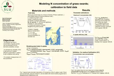
Materials and methods
Parameter estimations
Field data
Above ground biomass of a mixture of timothy
(Phleum pratense L.) and meadow fescue (Festuca
pratensis Huds.), in 2 seasonal growth cycles,
during 2 consecutive years, at 3 levels of
nitrogen application N0, N1 and N2 0, 140 and
200 kgN/ha/y), sampled at 7 site conditions in
Central and Southern Sweden, altogether 84
growth periods.
Maximum N concentration (N2)

Fig.4. nMax (g N/g d.w.) decreases with
increasing above ground biomass and decreasing
day length. nMax is determined by the
multiplicative effect of the response functions.
Example from Uppsala 1985-86.
Henrik Eckersten1 Bengt Torssell1 Alois
Kornher2 1Dept. of Ecology and Crop Production
Science, Swedish University of Agricultural
Sciences, Sweden (henrik.eckersten_at_evp.slu.se) 2In
stitute of Crop Science and Plant Breeding and
grassland and organic farming, CAU University of
Kiel, Germany
Polar circle
Climate in Uppsala Mean air temperature 17 oC
in July, 5 oC in January. Annual precipitation
is 500-600 mm.
N uptake efficiency (N0)
Fig.5 cAvailable ( per day) decreased after
cutting. x-axes Growth period 1-4. Example from
Uppsala 1985-86.

• Objectives
• To examine how well N concentration of grass
  swards can be predicted from the
  demandavailability concept.
• To estimate the variability of the N demand and N
  uptake efficiency parameters in relation to site
  conditions and cutting.
• To evaluate consequences on N flow predictions.
•  

Modeling plant daily N uptake
Growth period
At high N availability NUptake minimum of (0.04
. shoot growth 0.015 . root growth)
and (shoot biomass . (nMax - nShoot) root
biomass . (0.015 nRoot)) At low N
availability NUptake cAvailable . Soil mineral
N content
Validation for medium fertilisation (N1)
N concentration was overestimated.
Fig.6. Simulated (blue line) and observed
(crosses) shoot N concentration (g N/g d.w.) for
the medium fertilised stand. Red line
cAvailable is calibrated to N1. Example from
Uppsala 1985-86.
Fig.1. Approximate schematic description of N
dynamics of the N uptake model. Shoot and root
biomass, and soil mineral N, are simulated with
linked models programmed in Matlab/Simulink
(MathWorks Ltd).
2
1. Calibration of maximum N concentration nMax
Calibration of cAvailable for N1

• Conclusions
• - Decreasing maximum N concentration could be
  described as a combination of increasing biomass
  and decreasing day length.
• The N uptake efficiency decreased after cutting,
  and correlated with variations in radiation use
  efficiency.
• Maximum N concentration and, especially, N
  uptake efficiency need to be calibrated for new
  site conditions, to predict plant N uptake.

Fig.7 cAvailable( per day) was lower for N1
than N0 (average of all seven N1
treatments). Blue Calibrated for N0 Red
Calibrated for N1
Growth period
Fig.2. Simulated (line) and observed (crosses)
shoot N concentration (g N/g d.w.) for the high
fertilised stand (N2). One calibration for whole
period. Example from Uppsala 1985-86.
N uptake vs Radiation use efficiencies
Fig.8 yaxes cAvailable x-axes Radiation use
efficiency Both parameters are normalised to its
value of the first growth period. Radiation use
efficiency is defined as daily shoot growth per
intercepted global radiation, and was estimated
by calibration in a previous study. All seven N0
treatments.
2. Calibration of N uptake efficiency cAvailable
1
2
3
4
Fig. 3. Simulated (line) and observed (crosses)
shoot N concentration (g N/g d.w.) for the non
fertilised stand (N0). 1 4 are growth periods,
after winter or cutting. Calibration for each
growth period. Example from Uppsala 1985-86.
N0 no fertilisation N1 140 kgN/ha/y
(10040) N2 200 kgN/ha/y (12080) nMax
Maximum shoot N concentration (g
N/g d.w.) cUptake N uptake efficiency (1/d)
(Fraction of soil mineral N
taken up per day) nShoot, nRoot Actual
shoot and root N
concentrations (gN/gd.w.)
Importance of site specific calibration
Variation in N flows due to site variations in
parameter values
()
()
()
References to original model Eckersten, H.,
Blombäck, K., Kätterer, T., Nyman, P., 2001.
Modelling C, N, water and heat dynamics in winter
wheat under climate change in southern Sweden.
Agriculture Ecosystems and Environment. vol
86(3), pp 221-235 to Matlab/Simulink
application Eckersten, H., Noronha-Sannervik,
A., Nyman, P., Torssell, B., 2001. Modelling mass
flows in soil plant systems using
Matlab/Simulink. In Björneå, T.I., Ed. Nordic
MATLAB Conference Program Proceedings.
October 17-18, Oslo, Norway. ISBN 82-995955-0-9.
pp II44-49.
Fig. 10 Mean error in simulated N flows at
Uppsala N0 due to using cAvailable for other
sites. Range Uptake -50 to 3 Range Leaching
-9 to 26
Fig.11 Mean error in simulated N flows at Uppsala
N2 due to using nMax for other sites. Range
Uptake -24 to 0 Range Leaching 0 to 9
Fig. 9 Mean error in simulated N flows of N1 due
to using cAvailablefor N0. Fig 9-11 N flows
are accumulated during the first year.
3
Fig. 1. Schedule of the full model as programmed
in Matlab/Simulink (MathWorks Ltd), showing the
links between the plant model, water model and
soil nitrogen model. Air temperature (Ta),
relative air humidity (h), wind speed (u),
precipitation (P) and global radiation (Rs) are
weather inputs. RsInt is intercepted radiation,
JDN is Julian day number, LAI is leaf area index,
zr is root depth, Wr is root biomass, and SoilRWC
is soil relative water content.