
Multi-modal%20Adaptive%20Land%20Mine%20Detection%20Using - PowerPoint PPT Presentation
Title:
Multi-modal%20Adaptive%20Land%20Mine%20Detection%20Using
Description:
2. Sensor Phenomenology. 2.1 Ground Penetrating Radar (GPR) 2.2 ... 2.1 GPR Phenomenology (echo from air-ground interface) (echo from buried target) ... – PowerPoint PPT presentation
Number of Views:576
Avg rating:3.0/5.0
Title: Multi-modal%20Adaptive%20Land%20Mine%20Detection%20Using
1
DARPA-ARO MURI
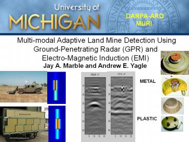
Multi-modal Adaptive Land Mine Detection
Using Ground-Penetrating Radar (GPR) and
Electro-Magnetic Induction (EMI)
Jay A. Marble and Andrew E. Yagle
METAL
PLASTIC
2
Outline
- Application Overview
- 1.1 Data Collection
- 1.2 Metal and Plastic Landmines
- 2. Sensor Phenomenology
- 2.1 Ground Penetrating Radar (GPR)
- 2.2 Electromagnetic Induction (EMI)
- 2.3 Overview of Approach
- 3. Metal Landmine Detection
- 3.1 GPR Signature Features
- 3.2 EMI Signature Features
- 4. Plastic Landmine Detection
- 4.1 Plastic Landmine Detection Difficulty
- 4.2 Hyperbola Flattening Transform
- 4.3 GPR Signature of Plastic Landmines
- 4.4 Metal Firing Pin Detection
- 5. Adapting to Changes in Environment
- 6. Current Progress
3
1. Application Overview1.1 Data Collection
USArmy Mine Hunter / Killer System
EMI Coils
GPR Antennae
EMI Facts
GPR Facts
Bandwidth 500MHz - 2GHz
Operating 75 Hz Frequency
Sampling Along Track 5cm (2) Cross
Track 15cm (6) Swath 3.0m
Sampling Along Track 5cm Cross Track
17.5cm Swath 2.8m
Depth Resolution Free Space - 10cm (4)
Soil (er3) - 5.7cm (2.3)
Database 11000m2
4
1. Application Overview1.1 Data Collection
5
1. Application Overview1.2 Metal Mines
Metal Landmines
Database Contains 70 metal cased mines buried
from 0 to 3 (Shallow).
93 metal cased mines buried from 3 to
6 (Deep).
Type M-15 Metal Casing Burial Depth 3 Width
13 Height 5.9
M-21 Metal Casing Burial Depth 1 Width
13 Height 8.1
Type TM-62M Metal Casing Burial Depth
2 Width 13 Height 5.9
6
1. Application Overview1.2 Plastic Mines
Plastic Landmines
Type TMA-4 Plastic Casing Burial Depth
2 Width 11 Height 4.3
Type TM-62P Plastic Casing Burial Depth
2 Width 13 Height 5.9
Database Contains 156 Shallow 265 Deep
Type VS1.6 Plastic Casing Burial Depth
6 Width 8.6 Height 3.5
Type VS2.2 Plastic Casing Burial Depth
1 Width 9 (.23m) Height 4.5 (.115m)
Type M-19 Plastic Width 0.33m Height 3.5
7
1. Application Overview
GOAL To determine presence vs. absence of land
mines vs. other metal objects USING Both GPR and
EMI data (multi-modal detection algorithm)
LANDMINES
NOT LANDMINES
How to discriminate between landmines and other
objects using GPR and EMI ?
8
Outline
- Application Overview
- 1.1 Data Collection
- 1.2 Metal and Plastic Landmines
- 2. Sensor Phenomenology
- 2.1 Ground Penetrating Radar (GPR)
- 2.2 Electromagnetic Induction (EMI)
- 2.3 Overview of Approach
- 3. Metal Landmine Detection
- 3.1 GPR Signature Features
- 3.2 EMI Signature Features
- 4. Plastic Landmine Detection
- 4.1 Plastic Landmine Detection Difficulty
- 4.2 Hyperbola Flattening Transform
- 4.3 GPR Signature of Plastic Landmines
- 4.4 Metal Firing Pin Detection
- 5. Adapting to Changes in Environment
- 6. Current Progress
9
2.1 GPR Phenomenology
Continuous, Stepped Frequency Radar 500MHz
1.5GHz 128 Frequency Steps
Tx
Rx
Antenna Module
h
Air
Fourier Transform
Transmit Pulse
Ground Interface
Layer 2
d
Target
...
Target
f1
f2
fN
f3
Sampled Frequencies
Depth Profile
m
10
2.1 GPR Phenomenology
(echo from air-ground interface)
(echo from buried target)
- GT Gain of transmit antenna
- GR Gain of receive antenna
- ER Electric field strength at the receiver
- E0 Transmitted Electric field strength.
- h Height of antenna above ground
- d Depth of target below the surface
- Wavelength in Free Space
- sRCS Target Radar Cross Section
(Propagation Constant Above the ground)
This model is for the antenna directly
above the buried object.
11
2.1 GPR Phenomenology
Slightly- Conducting Media Approximation
12
2.1 GPR Phenomenology
Data collected in time and space.
Synthetic Aperture
Antenna
Pattern
13
2.1 GPR Phenomenology
TM-62M Landmine
Unimaged Signature
TM-62M at 6
X
Metal Casing Height 6 Width 13 Depth
6
Z
14
2.2 EMI Phenomenology
Simplified EMI System Concept
Current Source
Data Storage
Electronics Sampler
Source H-field
Metal Object Reaction
Incident Field at Object
15
2.2 EMI Phenomenology
(x,y,h)
(x,y,-d)
Source H-field
16
2.2 EMI Phenomenology
Model assumes a solid spherical target.
Metal Object Reaction
17
2.2 EMI Phenomenology
Model no longer assumes a solid spherical
target.
Target Magnetic Polarizability Vector
H0x Horizontal magnetic field at the center of
the target produced by the source
magnetic dipole. Hxz Vertical magnetic field
at the receive coil produced by the
horizontal induced magnetic dipole. H0z
Vertical magnetic field at the center of the
target produced by the source
magnetic dipole. Hzz Vertical magnetic field
at the receive coil produced by the
vertical induced magnetic dipole.
18
2.2 EMI Phenomenology
EMI Spatial Signature
19
2.2 EMI Phenomenology
1 2 3 4 5 6 7 8 9 10 11 12 13 14 15 16
EMI Spatial Signature
Depth 1
Depth 3
Coil Number (Across Track)
Along Track
20
2.3 Overview of Approach
POI
Screener Points-of-Interest (POI) are detected
and reported. This stage must
be fast and must detect all landmines, but can
have false-alarms.
Features Aspects of the detected objects are
characterized in a vector of
feature values.
Discriminant Combines object features into a
test statistic.
21
2.3 Overview of Approach Screener Stage
Point-of- Interest List
22
2.3 Overview of Approach Feature Extraction
POI List
EMI Data
EMI Data
- Index X Location Y Location
- 291456.6558 4227053.1692
- 2 291382.6225 4227053.3659
- 3 291354.7422 4227052.5429
- .
- .
- .
- N 291309.1396 4227060.2448
4227052.5429
291354.7422
Feature Vector
GPR Features Depth Width Height RCS EMI
Features Magnetic Dipole Moments Decay Rates
To Discriminant Function
Extracted GPR Cube
Extracted EMI Chip
23
2.3 Overview of Approach Discriminant Function
Quadratic Polynomial Discriminant Function (Shown
here for 2 features.)
- The QPD can be thought of as
- a mapping. The feature vector
- (x1,x2) is mapped into a statistic
- s based on the training of the
- coefficients (c1,c2,c3,c4,c5,c6).
- The feature values are scalar
- numbers describing object
- X1 - Feature Value 1
- (Like object diameter)
- X2 Feature Value 2
- (Like object depth)
Output Statistic
24
Outline
- Application Overview
- 1.1 Data Collection
- 1.2 Metal and Plastic Landmines
- 2. Sensor Phenomenology
- 2.1 Ground Penetrating Radar (GPR)
- 2.2 Electromagnetic Induction (EMI)
- 2.3 Overview of Approach
- 3. Metal Landmine Detection
- 3.1 GPR Signature Features
- 3.2 EMI Signature Features
- 4. Plastic Landmine Detection
- 4.1 Plastic Landmine Detection Difficulty
- 4.2 Hyperbola Flattening Transform
- 4.3 GPR Signature of Plastic Landmines
- 4.4 Metal Firing Pin Detection
- 5. Adapting to Changes in Environment
- 6. Current Progress
25
3. Metal Mines Algorithm
Adaptive Environmental Parameter Estimation
EMI Data
EMI Polarization Vector Decay Rate
EMI Simple Threshold
Detection List
Y/N
W-k Imaging (Size/Depth)
POI Detector
GPR Data
Discriminant Function
Feature Extractor
Proposed Architecture for Metal Landmine Detection
26
3. Wavenumber Migration Imaging
Focused Point Target
Mechanics of Wavenumber Migration
Hyperbolic Point Target
Place in W-k Format
2D Phase Comp.
2D FFT
Stolt Interp.
2D
Azimuth
Stolt
2D
Phase
FFT
Interp
FFT
Comp
R(kx,W)
D(kx,kz)
R(kx,W)F(kx,,W)
27
3.1 GPR Signature
TM-62M Landmine
- Depth and Azimuth Resolution
- e r e r rd
- variation median
inches - Air 1 1 3.94
- Dry Sand 4-6 5 1.76
- Wet Sand 10-30 20 0.88
- Dry Clay 2-5 3 2.27
- Wet Clay 15-40 27 0.76
B 1.5GHz f0 1.25GHz Q 60
Metal Case Height 6 Width 13 Depth 6
28
3.1 GPR Signature
Unimaged Signature
- Signature before imaging
- is dominated by the
- standard hyperbola.
- Depth can be determined
- if data is properly
- calibrated. Size requires
- imaging to estimate.
- Convexity of signatures
- is determined by the
- speed of propagation
- in the medium.
Depth Inches
Along Track Inches
29
3.1 GPR Signature
- Imaged signature shows
- reflections from the top
- and bottom of the
- landmine.
- Length of the object can now
- be estimated from the
- length of the top and
- bottom reflections.
- Height of the object can be
- estimated from the distance
- between the two reflections.
- Depth has been calibrated
- during the imaging process.
Image
Depth Inches
Along Track Inches
30
3.1 GPR Signature
Image
- Estimated Depth and Size
- Depth 5.7
- Length 11.3
- Height 6.8
- Ground Truth
- Depth 6
- Length 13
- Height 6
13
6
Depth Inches
Top Reflection
Bottom Reflection
(Dry Clay)
Along Track Inches
About 3 res. cells across target in depth.
31
3.1 GPR Signature
Objects Reported
- Four objects are identified
- by setting a threshold and
- clustering connected pixels.
- Objects 1 and 2 are clearly
- above the ground and can
- be eliminated.
- Objects 3 and 4 are the top
- and bottom reflections.
2
1
3
Top Object
4
Depth Inches
Bottom Object
Along Track Inches
32
3.1 GPR Signature
Objects Reported
- Length is estimated by
- averaging the lengths
- of the two reflections.
- (Est. Length 11.3)
- Height is the distance
- between the two
- reflections.
- (Est. Height 6.8)
- Depth is the distance from
- the ground surface (0)
- to the top reflection.
- (Est. Depth 5.7)
10.8
5.7
6.8
Depth Inches
12.5
Along Track Inches
33
3.1 GPR Signature
Repeatability Study
Ten Signatures Before Imaging
34
3.1 GPR Signature
Repeatability Study
Ten Signatures After Imaging
35
3.1 GPR Signature
Repeatability Study
Ten Signatures Binarized
36
3.1 GPR Signature
Length inches
Height inches
Depth inches
Number
Repeatability Study
1 12 6.8 6.7
2 11.3 6.8 5.6
3 11.3 6.8 5.6
4 18 6.8 5.6
5 14 6.8 6.7
6 11.3 5.7 6.7
7 10.7 5.7 6.7
8 9.3 6.8 6.7
9 11.3 5.7 6.7
10 10.7 6.8 6.7
Note Depth Sample
Spacing 1.1
Ground Truth Depth 6
Length 13 Height 6
37
3.2 EMI Signature
Magnetic Polarizability
(signal model)
(N Samples)
(Least Squares Estimator)
- To compute the H matrix, we must
- know the depth of the target.
38
3.2 EMI Signature
- GPR (Radar) gives depth information
- EMI (Dipole models) give H matrix values
- Combining these Multi-modal detection
- Synergy Each helps the other work better
39
3.2 EMI Signature
40
3.2 EMI Signature
Aluminum Plate
Iron Sphere
No Target Present
Amps
Target Present
time
Decay Rate Discriminant
41
3.2 EMI Signature
- Sum of Decaying
- Exponentials (Prony)
- N2 is usually enough
- Decay Rate Features
42
3. Metal Mines Summary
EMI Features
GPR Features
- Magnetic Polarizability
- W-k Imaging Features
Depth Length Height
- Decay Rate Features
- Other Features
43
Outline
- Application Overview
- 1.1 Data Collection
- 1.2 Metal and Plastic Landmines
- 2. Sensor Phenomenology
- 2.1 Ground Penetrating Radar (GPR)
- 2.2 Electromagnetic Induction (EMI)
- 2.3 Overview of Approach
- 3. Metal Landmine Detection
- 3.1 GPR Signature Features
- 3.2 EMI Signature Features
- 4. Plastic Landmine Detection
- 4.1 Plastic Landmine Detection Difficulty
- 4.2 Hyperbola Flattening Transform
- 4.3 GPR Signature of Plastic Landmines
- 4.4 Metal Firing Pin Detection
- 5. Adapting to Changes in Environment
- 6. Current Progress
44
4. Plastic Mines Algorithm
Proposed Architecture for Plastic Landmine
Detection
Adaptive Environmental Parameter Estimation
EMI Data
EMI (Firing Pin)
HFT Detection Algorithm
Detection List
Y/N
GPR Data
W-k Imaging (Size/Depth)
POI Detector
Discriminant Function
Feature Extractor
45
4.1 Plastic Mine Detection
- The standard detection approach is to create
the plan view image - below by taking a standard deviation over
depth. - Using this statistic there are many false
alarms, but most mines - are detected. Deeply buried plastic mines,
however, are often missed.
GPR Standard Detection Statistic Standard
Deviation Over Depth Bins
46
4.1 Plastic Mine Detection
47
4.1 Plastic Mine Detection
ROC Curve
- About 80 of deep
- VS1.6 plastic mines
- are detectable.
Probability of Detection
Deeply Buried VS1.6 (Depth lt3)
Probability of False Alarm
48
4.1 Plastic Mine Detection
Surface
Plastic Landmine (VS1.6)
Top of Mine at 6
- Deeply buried plastic landmines face a low
signal-to-noise ratio (SNR). - Strata in the ground can create large radar
returns that lead to false alarms. - The Hyperbola Flattening Transform seeks to
exploit all the energy of the hyperbolic
signature.
Soil Stratum
49
4.2 Hyperbola Flattening
Mathematical Description
Remapping
Original Hyperbola
45 Rotation
Simulation
Simulation
Simulation
Simulation
- The Hyperbola Flattening Transform converts a
hyperbolic - signature into a straight line at 45.
50
4.2 Hyperbola Flattening
0
Application to Simulated Data
- The RADON transform
- creates projections by
- summing along lines.
- Projections are oriented
- for 0 to 180.
90
- Radon Transform of the
- flattened hyperbola has a
- strong maximum at 45
- corresponding to the energy
- contained in the hyperbola.
- Radon Transform illustration
- shows a projection for 120
- from a circle.
120
180
51
4.2 Hyperbola Flattening
Application to Simulated Data
52
4.2 Hyperbola Flattening
Application to Real Data
53
4.2 Hyperbola Flattening
Transform Location of Hyperbolic Signature
54
4.2 Hyperbola Flattening
55
4.2 Hyperbola Flattening
Algorithm Application
Original Image
- The HFT will now be
- applied as a detector.
- A small kernel is moved
- throughout the scene. At
- each location, the HFT is
- applied.,
- At each point the HFT is
- run for several values
- of the a parameter. The
- maximum result is placed
- into a detection image.
VS1.6
Depth
Along Track
56
4.2 Hyperbola Flattening
Algorithm Application
Hyperbola Detection Image
- The HFT is applied to all
- locations in the scene.
- The detection image shown
- here is the result.
- Bright pixels correspond
- to hyperbolas. Hyperbolic
- signatures have been
- contrast enhanced, while
- non-hyperbolas are
- suppressed.
VS1.6
Depth
Along Track
57
4.2 Hyperbola Flattening
Algorithm Application
Hyperbola-like Regions
- Pixels that break a certain
- threshold are shown.
- These pixels reveal the
- locations of the most
- hyperbola-like signals
- in the scene.
- The region corresponding
- to the VS1.6 has been
- enhanced by the HFT
- detector.
VS1.6
Depth
Along Track
58
4.3 GPR Signature
VS1.6 at 1
59
4.3 GPR Signature
M19 at 5
60
4.4 Firing Pin
EMI Data
Firing Pin Detection
1 2 3 4 5 6 7 8 9 10 11 12 13 14 15 16
Coil Number (Across Track)
Landmines contain a small amount of metal
in the firing pin. The data here has
been non- linearly altered. (That is, 3
square roots have been applied.)
Along Track
Plastic
Metal
Metal
61
4.4 Firing Pin
Firing Pin Detection
All These Landmines are Plastic. Nevertheless, an
EMI signal is attainable. The sensor sled was
lowered to just 2 above the ground.
EMI Spatial Signature
EMI Spatial Signature
EMI Spatial Signature
TM-62P at 2
VS1.6 at 1
VS2.2 at 1
62
4. Plastic Mine Summary
EMI Features
GPR Features
- Firing Pin Detection (binary)
(detected)
- W-k Imaging Features
(not-detected)
Depth? Length Height
- Magnetic Polarizability
- Other Features
- Decay Rate Features
63
Outline
- Application Overview
- 1.1 Data Collection
- 1.2 Metal and Plastic Landmines
- 2. Sensor Phenomenology
- 2.1 Ground Penetrating Radar (GPR)
- 2.2 Electromagnetic Induction (EMI)
- 2.3 Overview of Approach
- 3. Metal Landmine Detection
- 3.1 GPR Signature Features
- 3.2 EMI Signature Features
- 4. Plastic Landmine Detection
- 4.1 Plastic Landmine Detection Difficulty
- 4.2 Hyperbola Flattening Transform
- 4.3 GPR Signature of Plastic Landmines
- 4.4 Metal Firing Pin Detection
- 5. Adapting to Changes in Environment
- 6. Current Progress
64
5. Adapting to Environmental Changes
Ei
- Reflection Coefficient
R12
Es
Ei
Es
- Measuring Dielectric Constant
- of a material is done using the
- reflection coefficient.
e1 e0
- er is frequency independent
- for 500 MHz lt f lt 2.0GHz
e2 er e0
- e r e
r - variation
median - Air 1
1 - Dry Sand 4-6 5
- Wet Sand 10-30 20
- Dry Clay 2-5 3
- Wet Clay 15-40 27
Et
65
5. Adapting to Environmental Changes
- Solving for er is non-linear
- Therefore, estimates of
- er are very sensitive to noise
- in the observations of R12.
Reflection Coefficient
66
5. Adapting to Environmental Changes
Example Dry Soil (er small)
- Reflection Coefficient for 128 Frequencies is
contaminated with - Gaussian Noise.
- Variance at a single frequency is large, so all
128 must be combined - in some way to reduce the estimate
variance.
nN(0,0.01) (SNR 10dB)
After Conversion to er
nX1?(0,3.6)
Sample Mean Biased Estimate
128 Frequencies
67
5. Adapting to Environmental Changes
Estimate From 128 Frequencies
Adaptive Filter Output
- Simple First Attempt at Adaptive Filter
- Averages er of 50 locations along track
- Performed acceptably for er 4
68
5. Adapting to Environmental Changes
Approach to Adaptive Processing of er Changes
- Estimation of er is a challenge.
- Utilize all available information
- 128 Frequencies
- 20 Antennas
- Multiple Locations Along Track
- Characterize Noise after Conversion to er
- Xi er ni n? (How is n
distributed?)
- Determine Unbiased Estimator for er given
non-Gaussian - nature of noise using 128 frequencies (maximum
likelihood) - Possibly incorporate a priori information (max.
a posteriori)
69
Outline
- Application Overview
- 1.1 Data Collection
- 1.2 Metal and Plastic Landmines
- 2. Sensor Phenomenology
- 2.1 Ground Penetrating Radar (GPR)
- 2.2 Electromagnetic Induction (EMI)
- 2.3 Overview of Approach
- 3. Metal Landmine Detection
- 3.1 GPR Signature Features
- 3.2 EMI Signature Features
- 4. Plastic Landmine Detection
- 4.1 Plastic Landmine Detection Difficulty
- 4.2 Hyperbola Flattening Transform
- 4.3 GPR Signature of Plastic Landmines
- 4.4 Metal Firing Pin Detection
- 5. Adapting to Changes in Environment
- 6. Current Progress
70
6. Current Progress
- Wavenumber Migration Processor
GPR - Point Target Simulator
- Successful Imaging of Metal Landmines
- Successful Imaging of Plastic Landmines
- GPR Feature Set
- Identify Metal Landmine GPR Feature Set
- Identify Plastic Landmine GPR Feature
Set - Automated Extraction of GPR Metal Features
- Automated Extraction of GPR Plastic
Features - Plastic Landmine Detection
- Evaluate Baseline Performance with
ROC Curve - Implement the Hyperbola Flattening
Transform - Enhance Processing Speed of the HFT
- Evaluate HFT Performance using ROC
Curves
71
6. Current Progress
- Physical Signal Modeling
EMI - Simple Target Simulator (dipole induction)
- Study effect of soil conductivity on
measured signature. - EMI Feature Set
- Identify Metal Landmine EMI Feature Set
- P Use Least Squares to Estimate Magnetic
Polarization Features - P Measure decay rates of iron and aluminum
objects. - Identify Firing Pin Detection Features
- Spectral Noise Whitener for Firing Pin
Detection - Automated Extraction of EMI Metal
Features - Automated Extraction of EMI Firing Pin
Features
72
6. Current Progress
Adaptive Estimation of er Estimation of er
from GPR scattering measurements. Determine
statistical model of noise in er observations.
Investigate MLE and MAP estimators for er
Recommended
CrystalGraphics Presentations


