Oligopoly Models

1
Oligopoly Models

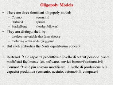
• There are three dominant oligopoly models
• Cournot (quantity)
• Bertrand (price)
• Stackelberg (leader-follower)
• They are distinguished by
• the decision variable that firms choose
• the timing of the underlying game
• But each embodies the Nash equilibrium concept
• Bertrand ? Se capacità produttiva e livello di
  output possono essere modificati facilmente (es.
  software, servizi bamcari/assicurativi)
• Cournot ? se è più costoso modificare il livello
  di produzione o la capacità produttiva (cemento,
  acciaio, automobili, computer)

2
Matrice dei profitti in un gioco sulle quantità
prodotte (Cournot)

3
Cournot example American and United

• Q 339 P demand function
• MC 147 marginal cost
• qA Q(P) qU (339 P) qU demand for A
• qU Q(P) qA (339 P) qA demand for U
• P 339 qA qU inverse demand function
• MRA 339 2qA qU marginal revenue for A
• MRU 339 2qU qA marginal revenue for U
• Max profit ? MR MC
• 339 2qA qU 147
• qA 96 1/2 qU best response function for A
• qU 96 1/2 qA best response function for U
• qA 96 1/2 (96 1/2qA)
• qA 64 qU 64
• Q qA qU 128 P 339 Q 211

4
Monopolio Output che max il profitto per
American Airlines
(a) Monopolio
p
, per
passeggero
339
243
MC
147
D
MR
0
339
169.5
96
q
, Migliaia di passeggeri American Airlines
A
Per quadrimestre
5
Duopolio Output che max il profitto per
American Airlines
(b) Duopolio
p
, per
passeggero
339
275
211
MC
147
q

64
U
r
r
MR
D
D
0
339
275
137.5
64
128
q
, Migliaia di passeggeri American Airlines
A
per quadrimestre
6
Curve di reazione di American e United
q
, United, migliaia
U
di passeggeri per quadr.
192
Curva di reazione di American
96
Equilibrio di Cournot
64
48
Curva di reazione di United

0
192
96
64
q
, American, migliaia di
A
passeggeri per quadrimestre
7
Duopoly Equilibria
(a) Equilibrium Quantities
q
, Thousand United
U
passengers per quarter
192
American

s best-response curve
Contract
curve
Price-taking equilibrium
96
Cournot equilibrium
64
Stackelberg equilibrium
48
Cartel
United

s best-response curve
equilibrium
0
192
96
64
48
q
, Thousand American passengers per quarter
A
8
Cournot equilibrium and the number of firms

• MR P(1 1/?r) ?r elasticity of the residual
  demand curve
• ?r n? ? market elasticity of demand
• n number of competing firms
• MR P(1 1/n?) MC
• n 1 ? monopoly
• n 8 ? perfect competition
• Lerner Index (P MC) / P - 1 / n?

9
Cournot Equilibrium Varies with the Number of
Firms

10
The Cournot Model

• Start with a duopoly
• Two firms making an identical product (Cournot
  supposed this was spring water)
• Demand for this product is

P A - BQ A - B(q1 q2)
where q1 is output of firm 1 and q2 is output of
firm 2

• Marginal cost for each firm is constant at c per
  unit
• To get the demand curve for one of the firms we
  treat the output of the other firm as constant
• So for firm 2, demand is P (A - Bq1) - Bq2

11
The Cournot model (cont.)
If the output of firm 1 is increased the demand
curve for firm 2 moves to the left
P (A - Bq1) - Bq2

The profit-maximizing choice of output by firm 2
depends upon the output of firm 1
A - Bq1
A - Bq1
Marginal revenue for firm 2 is
Solve this for output q2
Demand
c
MC
MR2 (A - Bq1) - 2Bq2
MR2
MR2 MC
q2
Quantity
A - Bq1 - 2Bq2 c
? q2 (A - c)/2B - q1/2
12
The Cournot model (cont.)
q2 (A - c)/2B - q1/2
This is the best response function for firm 2
It gives firm 2s profit-maximizing choice of
output for any choice of output by firm 1
There is also a best response function for firm 1
By exactly the same argument it can be written
q1 (A - c)/2B - q2/2
Cournot-Nash equilibrium requires that both firms
be on their best response functions.
13
Cournot-Nash Equilibrium
q2
The best response function for firm 1 is q1
(A-c)/2B - q2/2
If firm 2 produces (A-c)/B then firm 1 will
choose to produce no output
The Cournot-Nash equilibrium is at Point C at the
intersection of the best response functions
(A-c)/B
Firm 1s best response function
If firm 2 produces nothing then firm 1 will
produce the monopoly output (A-c)/2B
The best response function for firm 2 is q2
(A-c)/2B - q1/2
(A-c)/2B
C
qC2
Firm 2s best response function
q1
(A-c)/2B
(A-c)/B
qC1
14
Cournot-Nash Equilibrium
q1 (A - c)/2B - q2/2
q2
q2 (A - c)/2B - q1/2
(A-c)/B
? q2 (A - c)/2B - (A - c)/4B q2/4
Firm 1s best response function
? 3q2/4 (A - c)/4B
(A-c)/2B
? q2 (A - c)/3B
C
(A-c)/3B
? q1 (A - c)/3B
Firm 2s best response function
q1
(A-c)/2B
(A-c)/B
(A-c)/3B
15
Cournot-Nash Equilibrium (cont.)

• In equilibrium each firm produces qC1 qC2 (A
  - c)/3B
• Total output is, therefore, Q 2(A - c)/3B
• Recall that demand is P A - BQ
• So the equilibrium price is P A - 2(A - c)/3
  (A 2c)/3
• Profit of firm 1 is (P - c)qC1 (A - c)2/9
• Profit of firm 2 is the same
• A monopolist would produce QM (A - c)/2B
• Competition between the firms causes their total
  output to exceed the monopoly output. Price is
  therefore lower than the monopoly price
• But output is less than the competitive output (A
  - c)/B where price equals marginal cost and P
  exceeds MC

16
Numerical Example of Cournot Duopoly

• Demand P 100 - 2Q 100 - 2(q1 q2) A
  100 B 2
• Unit cost c 10
• Equilibrium total output Q 2(A c)/3B 30
• Individual Firm output q1 q2 15
• Equilibrium price is P (A 2c)/3 40
• Profit of firm 1 is (P - c)qC1 (A - c)2/9B
  450
• Competition Q (A c)/B 45 P c 10
• Monopoly QM (A - c)/2B 22.5 P 55
• Total output exceeds the monopoly output, but is
  less than the competitive output
• Price exceeds marginal cost but is less than the
  monopoly price

17
Cournot-Nash Equilibrium (cont.)

• What if there are more than two firms?
• Much the same approach.
• Say that there are N identical firms producing
  identical products
• Total output Q q1 q2 qN
• Demand is P A - BQ A - B(q1 q2 qN)
• Consider firm 1. Its demand curve can be
  written

This denotes output of every firm other than firm
1
P A - B(q2 qN) - Bq1

• Use a simplifying notation Q-1 q2 q3 qN

• So demand for firm 1 is P (A - BQ-1) - Bq1

18
The Cournot model (cont.)
If the output of the other firms is increased the
demand curve for firm 1 moves to the left
P (A - BQ-1) - Bq1

The profit-maximizing choice of output by firm 1
depends upon the output of the other firms
A - BQ-1
A - BQ-1
Marginal revenue for firm 1 is
Solve this for output q1
Demand
c
MC
MR1 (A - BQ-1) - 2Bq1
MR1
MR1 MC
q1
Quantity
A - BQ-1 - 2Bq1 c
? q1 (A - c)/2B - Q-1/2
19
Cournot-Nash Equilibrium (cont.)
q1 (A - c)/2B - Q-1/2
As the number of firms increases output of each
firm falls
How do we solve this for q1?
The firms are identical. So in equilibrium
they will have identical outputs
? Q-1 (N - 1)q1
As the number of firms increases aggregate
output increases
? q1 (A - c)/2B - (N - 1)q1/2
As the number of firms increases price tends
to marginal cost
As the number of firms increases profit of each
firm falls
? (1 (N - 1)/2)q1 (A - c)/2B
? q1(N 1)/2 (A - c)/2B
? q1 (A - c)/(N 1)B
? Q N(A - c)/(N 1)B
? P A - BQ (A Nc)/(N 1)
Profit of firm 1 is P1 (P - c)q1
(A - c)2/(N 1)2B
20
Concentration and Profitability

• Assume that we have N firms with different
  marginal costs
• We can use the N-firm analysis with a simple
  change
• Recall that demand for firm 1 is P (A - BQ-1) -
  Bq1
• But then demand for firm i is P (A - BQ-i) -
  Bqi
• Equate this to marginal cost ci

But Q-i qi Q and A - BQ P
A - BQ-i - 2Bqi ci
This can be reorganized to give the equilibrium
condition
A - B(Q-i qi) - Bqi - ci 0
? P - Bqi - ci 0
? P - ci Bqi
21
Concentration and profitability (cont.)
The price-cost margin for each firm is determined
by its own market share and overallmarket demand
elasticity
P - ci Bqi
Divide by P and multiply the right-hand side by
Q/Q
The verage price-cost margin is determined by
industryconcentration as measured by the
Herfindahl-Hirschman Index
P - ci
BQ
qi

P
P
Q
But BQ/P 1/? and qi/Q si
P - ci
si
so

?
P
Extending this we have
P - c
H

P
?
22
Misura della concentrazione

• Le industrie presentano strutture molto
  differenti
• Numero e distribuzione dimensionale delle imprese
• cereali da colazione alta concentrazione
• ristoranti bassa concentrazione
• Come misurare la struttura di mercato
• misura riassuntiva
• la curva di concentrazione è possibile
• preferenza per un numero singolo
• Rapporto di concentrazione o Indice di
  Herfindahl-Hirschman

23

• Indice di Herfindahl-Hirschman
• Informazioni sulle quote di mercato di tutte le
  imprese e non solo di quelle più grandi.
• HH ? si2
• si quota di mercato impresa i-esima
• Somma dei quadrati delle quote di mercato delle
  imprese del settore.

24
Misura della concentrazione

• Confronto tra due diverse misure della
  concentrazione

Imprese Quota mercato Quota di
mercato ordinate () al
quadrato
1 25
25
625
2 25
25
625
3 25
25
625
4 5
5
25
5 5
25
6 5
25
7 5
25
8 5
25
CR4 80
Indice di concentrazione
HH 2.000
25

• Lindice di concentrazione è influenzato da,
  esempio, fusioni

Imprese Quota mercato Quota di
mercato ordinate () al
quadrato
1 25
Esempio imprese 4 e 5 decidono di fondersi
25
Cambiamento quota di mercato
625
2 25
25
625
3 25
25
625
4 5
5
25



100
10
5 5
25
6 5
Lindice di concentrazione cambia
25
7 5
25
8 5
25
CR4 80
Indice di concentrazione
HH 2.000
85
2.050
26
(No Transcript)