A' Vector Analysis

1
Basic Antenna Theory

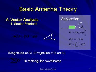
• Application

• A. Vector Analysis
• 1. Scalar Product

2

• 2. Vector Product

3

• 3. Circulation

Circulation of
Closed path
4

• 4. Flux

5

• 5. Gradient

(Rect. Coord.)
Del Operator
6

• 6. Divergence

ROC of a Field in Direction of Field
7

• 7. Curl

8
Rect. Coord.
Curl is a measure of fields ability to produce
torque
9
8. Laplacian
Rect. Coord.
10
9. Helmholtz Theorem
A vector is completely defined if its DIV Curl
are specified if the field vanished as r?h (or
if normal component is specified over some closed
surface) Note, we specified that DIV Curl are
ROCs are related to sources of the field.
Thus a vector field is specified by its vector
scalar source.
11
10. Divergence Theorem
12
10. Stokes Theorem
13
B. Maxwells Equations 1. Gauss Law
14
Line of Charge
For a Closed Surface
15
Apply Divergence Theorem
Maxwell Eqn. (Gauss Law for Points)
16
2. Amperes Law
17
For a very long straight wire,
lines encircle conductor
In this case,
18
3. Potential
19
Conservative Field
And
Grad. of a scalar
From
To find V from
a collection of charges
?
20
For general situations
where
Now, you can get from
21
4. Equation of Continuity
Current
Closed Surface Around One Plate
Current Entering Closed Surface
22
For I out of closed surface
By Divergence Theorem
Equation of Continuity
23
Returning to Amperes Law
In General Maxwell Equation
Current density is composed of two parts
24
5. Gauss Law for Magnetics
25
6. Faradays Law
Apply Stokes Thm
26
7. M.E. and Sources of Fields
27
8. Magnetic Vector Potential
28
(No Transcript)
29
9. Poynting Vector and Power
Outward Power Flow
From Stored Magnetic Electric Energies
30
Instantaneous Poynting Vector
31
C. Radiation
(Assume sinusoidal time variation)
1. Total
the gradient of a scalar
Scalar Potential from Charges
32
2. Wave Equations
From
Get
And
(sometimes called ß)
33
Looks messy, but note we still have not
specified yet. If we choose
Lorentz Gauge Condition
(which is really just the equation of continuity
in disguise!)
we get
34
And for single source notation
35
Solutions to Wave Eqns. Are Found by
Considering a Point Source (called a free-space
Greens Function
observation pt.
source pt.
is the wave eqn. for G
(this you can show with lots of effort)
36
We then deduce
convolution integral
Potential integrals are solutions to wave
equation!!
37
3. Elementary Source
We will now solve a most simple antenna and use
it as a building block (in our computer modeling)
to solve complicated antennas.
Short Electric Dipole, Constant (uniform) I
How short is short ? Why is it called a
Dipole? How can you achieve uniform I ?
38
dipole moment
39
Find from using sph.
coordinates.

40
1/r 1/r2
1/r3 Far Out Close In Real Close In
41
3 Regions
42
Far Field
In-phase terms Ratio of ? 1/r2 power variation
Magnitude of plane wave
Plane wave
Spherical wave!
43
Radially outward and variation No loss of
power, just spreads out
, N-S , E-W
Strongest at Equator Zero at Poles
Up close looks like a plane wave
44
Near and Fresnel
Usually lumped together into near field
90o out of phase with Energy oscillates
in out and is capacitive
(Near fields tied to J, P. Far fields tied to
displacement current)
45
(No Transcript)
46
Near Antenna
E H out of phase H in phase with I E in phase
with Q on ends
Far from Antenna
Never returns E in phase with H
P
47
Einduction Eradiation are 180o out of
phase Hinduction Hradiation are 90o out of
phase Why?
48

• D. Antenna Concepts

1.
Antennas are field warpers which transform
transmission line fields into spherical waves
with prefered directions and vice
versa. Antennas made of wires (linear antennas)
have currents and charges on them and if you know
or can guess I Q, you can find the far out
stuff via potential integrals (solutions to the
wave equation).
2.
49
If you dont know I or Q, you have lots of
hard work to do, because all you have is a
source function and conducting surface where E
is perpendicular to surface and Etangential is
zero. You then have to write a boundary value
equation to force Etan 0 at the conductors by
writing Etan in terms of where K is a
Greens function. The problem then is to find I
which is unfortunately inside the .
3.
50
Once you have E, H you can use S to get the
total power radiated over a sphere and define
4.
51
(No Transcript)
52
Patterns are usually plotted as a cross section
of the 3D surface in a plane. Often we choose
the planes as perpendicular cuts through the main
beam (maximum lobe).
E Plane Contains axis of main beam and
vector
H Plane Contains axis of main beam and
vector
53
Toroidal Shaped
Could plot fields too,
54
Gain and Directivity are dependent on . A
maximum (constant) value is often specified
6.
55
In general
for measurements
Antenna
(same r)
56
(No Transcript)
57
(No Transcript)
58
(No Transcript)
59
Since
60
Far field
GT, GR are often off-frequency
What about near field coupling? Tough! Got to
use network concepts.
61
Note how super-simple idealized the short
dipole is how complex the solution was. We
could do the same set-up for the next simplest
antenna, a ?/2 dipole but would find we would
have to integrate the assumed current to find
. Anything more complex than that we would
have to know the current and be able to
integrate it.
There is another possibility We could treat
complex structures as a collection of short
dipoles of different but uniform currents!
62
Looks simpler and it is but you must know or
guess I( l). IF you cant do this, you must
develop an integral equation for I.
63

• D. Integral Equation Formulation

The typical linear antenna is a cylindrical
dipole
L/2
2a
Z0
Gap is fed by
-L/2
field or Vo v. generator
64
(No Transcript)
65
Apply surface boundary condition
With Greens Function Notation,
with
66
Reduce volume to surface by assuming perfect
conductor applying axial symmetry it is OK to
consider just one value of
Pocklingtons Eqn.
67
Look at Kernel
It has a singularity of third order at and
the integration is over a surface, thus the
integral diverges, and Pocklingtons Eqn. cannot
be used for numerical analysis. This does not
make the integral equation meaningless. If the
THIN WIRE APPROXIMATION is applied
68
And observation points are taken along a line on
the cylinder surface so that
We get
Pocklingtons Thin Wire Equation